Curve fitting

[stellanhakansson]

I have a data set showing survival of preterm infants by gestational age in days (d154-195). Excel gives a logarithmic trend line which seems to fit nicely, but the equation <y=22.22ln(x)+12.752> given for the line doesn't produce the y-values I expect by entering 'x'. I would be grateful for some advice.

All the best,
Stellan Hakansson

 

[KRice]

I'm puzzled by the trendline shown in your plot. I don't see the same extent of curvature and the fit is not very good. One issue I see is related to the representation of the y data, described as a survival percentage. Excel will treat 9 % as 0.09. I can't tell from the image included in your post what values are actually being used. Is the first y value about 9.09 or 0.0909? This becomes an issue because of the relative disparity when the numerical representations of x differ by two orders of magnitude and they are being multiplied by ln(x), which will have a value of approximately 5 over the entire range represented here.

Book1
	H	I	J	K	L	M	N	O
1							2.546680906	-12.38901459
2	Observed Survival_%(y)		GA_d (x)	Observed Survival (y)	Original Estimated y=22.22ln(x)+12.752	Semi-Log Regression (ln-lin)	0.228230629	1.177663775
3	9.090909091		154	0.090909091	124.6730868	0.438496426	0.756852405	0.103088872
4	28.57142857		155	0.285714286	124.8169061	0.454979855	124.5091331	40
5	46.15384615		156	0.461538462	124.9598005	0.471357281	1.323197837	0.425092619
6	30.76923077		157	0.307692308	125.1017818	0.487630057
7	54.16666667		158	0.541666667	125.2428616	0.503799514
8	52		159	0.52	125.3830514	0.519866955
9	69.23076923		160	0.692307692	125.5223622	0.535833659
10	60		161	0.6	125.660805	0.551700881
11	46.15384615		162	0.461538462	125.7983906	0.567469853
12	70.58823529		163	0.705882353	125.9351295	0.583141785
13	72.4137931		164	0.724137931	126.071032	0.598717864
14	64.86486486		165	0.648648649	126.2061084	0.614199254
15	78.26086957		166	0.782608696	126.3403687	0.629587101
16	76.19047619		167	0.761904762	126.4738225	0.644882528
17	58.82352941		168	0.588235294	126.6064796	0.660086638
18	70		169	0.7	126.7383494	0.675200516
19	80		170	0.8	126.8694413	0.690225226
20	62.16216216		171	0.621621622	126.9997642	0.705161813
21	76.31578947		172	0.763157895	127.1293273	0.720011307
22	75		173	0.75	127.2581392	0.734774716
23	77.27272727		174	0.772727273	127.3862087	0.749453032
24	82.85714286		175	0.828571429	127.5135443	0.764047232
25	91.42857143		176	0.914285714	127.6401544	0.778558274
26	84.61538462		177	0.846153846	127.7660471	0.792987099
27	100		178	1	127.8912305	0.807334635
28	82.75862069		179	0.827586207	128.0157126	0.821601793
29	77.27272727		180	0.772727273	128.1395012	0.835789467
30	87.23404255		181	0.872340426	128.262604	0.849898538
31	87.75510204		182	0.87755102	128.3850286	0.863929874
32	85.71428571		183	0.857142857	128.5067823	0.877884324
33	86.66666667		184	0.866666667	128.6278725	0.891762729
34	94.23076923		185	0.942307692	128.7483064	0.905565911
35	91.83673469		186	0.918367347	128.8680911	0.919294682
36	91.4893617		187	0.914893617	128.9872335	0.932949841
37	96.875		188	0.96875	129.1057404	0.946532171
38	90.90909091		189	0.909090909	129.2236187	0.960042446
39	88		190	0.88	129.3408749	0.973481427
40	93.33333333		191	0.933333333	129.4575156	0.986849861
41	97.14285714		192	0.971428571	129.5735472	1.000148486
42	96.77419355		193	0.967741936	129.688976	1.013378027
43	95.77464789		194	0.957746479	129.8038083	1.026539198
44	91.78082192		195	0.917808219	129.9180502	1.039632702
Sheet1

Cell Formulas
Range	Formula
N1:O5	N1	=LINEST(K3:K44,LN(J3:J44),1,1)
K3:K44	K3	=H3/100
M3:M44	M3	=$N$1*LN(J3)+$O$1
Dynamic array formulas.

 

[stellanhakansson]

Hi, Many thanks for advice and time spent. Actually I don't expect survival to be linear to gestational age (gradually improving by GA), and I tried instead a polynomial trend line giving R2 close to .9. I think that will do.
Best, Stellan

 

[KRice]

Hi Stellan,

I wouldn't necessarily expect a linear trend either. I can't tell if that comment is due to my use of the LINEST function(?), but LINEST can be used to return the coefficients for many types of regression. In my last post, I used it for your original log-linear approach, and below I've extended it to perform a 2nd order polynomial regression and a linear regression. I am not surprised that log-linear (of the form y=a*ln(x) + c and shown in red) is very close to linear (of the form y = m*x + b and shown in blue)...that was the point I was making about the natural log of x over the domain shown. The range represented by ln(150) and ln(200) is [5.01, 5.3] -- hardly any variation at all -- and when multiplied by a coefficient (constant), there is very little variation in the first term of the log-lin model, so it appears to be nearly linear. Comparing the two curves on the plot confirms this. In the results delivered by LINEST, I've shown the fit coefficients in bold font and the R2 fit metric also in bold font.

Ideally, some underlying theory of the phenomena being investigated would offer insight into the model form used for regression. Given the biological nature of the data and assuming the data are representative of a single species, early deaths would shift the health of the gestating population upward (generally better health) and the number of premature deaths would therefore continue to decline. So I would expect the survivability rate to continuously increase, but at a lower rate, as a function of increasing gestational age until perhaps late term risks become significant and survivability might then decrease. I don't see clear indications in the data shown that such a downturn is real at very late gestational ages.

I would hesitate to apply a polynomial model to the data as it has the potential to introduce inflection points around which the local slope of the curve changes. These changes might be difficult to explain, and in some cases, the slope changes may defy logic. In any case, I suspect the preferred distributional models to consider for these data are found in survivability theory or reliability theory.

MrExcel_20230604.xlsx
	H	I	J	K	L	M	N	O	P	Q	R
1									Regression Analysis
2	Observed Survival_%(y)		GA_d (x)	Observed Survival (y)	Original Estimated y=22.22ln(x)+12.752	Semi-Log Regression (ln-lin)	Polynomial 2o Regression	Linear Regression	Semi-Log (ln-lin)
3	9.090909091		154	0.090909091	124.6730868	0.438496426	0.318202864	0.453744489	2.546680906	-12.38901459
4	28.57142857		155	0.285714286	124.8169061	0.454979855	0.352518498	0.468224764	0.228230629	1.177663775
5	46.15384615		156	0.461538462	124.9598005	0.471357281	0.385842365	0.482705039	0.756852405	0.103088872
6	30.76923077		157	0.307692308	125.1017818	0.487630057	0.418174463	0.497185313	124.5091331	40
7	54.16666667		158	0.541666667	125.2428616	0.503799514	0.449514794	0.511665588	1.323197837	0.425092619
8	52		159	0.52	125.3830514	0.519866955	0.479863356	0.526145862
9	69.23076923		160	0.692307692	125.5223622	0.535833659	0.509220151	0.540626137	Polynomial (2nd order)
10	60		161	0.6	125.660805	0.551700881	0.537585177	0.555106412	-0.000495884	0.187543789	-16.80315582
11	46.15384615		162	0.461538462	125.7983906	0.567469853	0.564958435	0.569586686	9.89452E-05	0.034548491	3.004223678
12	70.58823529		163	0.705882353	125.9351295	0.583141785	0.591339926	0.584066961	0.841881771	0.08419096	#N/A
13	72.4137931		164	0.724137931	126.071032	0.598717864	0.616729649	0.598547235	103.8254386	39	#N/A
14	64.86486486		165	0.648648649	126.2061084	0.614199254	0.641127603	0.61302751	1.471853864	0.276436591	#N/A
15	78.26086957		166	0.782608696	126.3403687	0.629587101	0.66453379	0.627507785
16	76.19047619		167	0.761904762	126.4738225	0.644882528	0.686948208	0.641988059	Linear
17	58.82352941		168	0.588235294	126.6064796	0.660086638	0.708370859	0.656468334	0.014480275	-1.776217799
18	70		169	0.7	126.7383494	0.675200516	0.728801741	0.670948608	0.001356946	0.237357593
19	80		170	0.8	126.8694413	0.690225226	0.748240856	0.685428883	0.740048812	0.106591531
20	62.16216216		171	0.621621622	126.9997642	0.705161813	0.766688202	0.699909158	113.8750419	40
21	76.31578947		172	0.763157895	127.1293273	0.720011307	0.784143781	0.714389432	1.293820274	0.454470182
22	75		173	0.75	127.2581392	0.734774716	0.800607591	0.728869707
23	77.27272727		174	0.772727273	127.3862087	0.749453032	0.816079634	0.743349981
24	82.85714286		175	0.828571429	127.5135443	0.764047232	0.830559909	0.757830256
25	91.42857143		176	0.914285714	127.6401544	0.778558274	0.844048415	0.772310531
26	84.61538462		177	0.846153846	127.7660471	0.792987099	0.856545154	0.786790805
27	100		178	1	127.8912305	0.807334635	0.868050124	0.80127108
28	82.75862069		179	0.827586207	128.0157126	0.821601793	0.878563327	0.815751354
29	77.27272727		180	0.772727273	128.1395012	0.835789467	0.888084762	0.830231629
30	87.23404255		181	0.872340426	128.262604	0.849898538	0.896614428	0.844711903
31	87.75510204		182	0.87755102	128.3850286	0.863929874	0.904152327	0.859192178
32	85.71428571		183	0.857142857	128.5067823	0.877884324	0.910698458	0.873672453
33	86.66666667		184	0.866666667	128.6278725	0.891762729	0.91625282	0.888152727
34	94.23076923		185	0.942307692	128.7483064	0.905565911	0.920815415	0.902633002
35	91.83673469		186	0.918367347	128.8680911	0.919294682	0.924386242	0.917113276
36	91.4893617		187	0.914893617	128.9872335	0.932949841	0.9269653	0.931593551
37	96.875		188	0.96875	129.1057404	0.946532171	0.928552591	0.946073826
38	90.90909091		189	0.909090909	129.2236187	0.960042446	0.929148114	0.9605541
39	88		190	0.88	129.3408749	0.973481427	0.928751869	0.975034375
40	93.33333333		191	0.933333333	129.4575156	0.986849861	0.927363855	0.989514649
41	97.14285714		192	0.971428571	129.5735472	1.000148486	0.924984074	1.003994924
42	96.77419355		193	0.967741936	129.688976	1.013378027	0.921612525	1.018475199
43	95.77464789		194	0.957746479	129.8038083	1.026539198	0.917249208	1.032955473
44	91.78082192		195	0.917808219	129.9180502	1.039632702	0.911894122	1.047435748
Sheet1

Cell Formulas
Range	Formula
M3:M44	M3	=$P$3*LN(J3)+$Q$3
N3:N44	N3	=$P$10*J3^2+$Q$10*J3+$R$10
O3:O44	O3	=$P$17*J3+$Q$17
P3:Q7	P3	=LINEST(K3:K44,LN(J3:J44),1,1)
P10:R14	P10	=LINEST(K3:K44,J3:J44^{1,2},1,1)
P17:Q21	P17	=LINEST(K3:K44,J3:J44,1,1)
K3:K44	K3	=H3/100
Dynamic array formulas.

 

[Tetra201]

@ stellanhakansson: To me, it looks like a classic case of y=c-2^((a-x)/b).
The best fit is achieved with a=150.1493, b=7.811379, c=0.945035, R2=0.866651.
I think, however, that c should be set to the actual survival rate of full-term neonates (probably, around 0.98).
Good luck with your research!

 

[stellanhakansson]

Hi,
Thank you for replies and bringing my question to higher levels. Much appreciated. I am still puzzled by the fact that Excel creates two different trend lines if the same data is depicted in a line-diagram or in a scatter-plot. The trend line of the line-diagram agrees well with my clinical impression, in that very few babies born at the limit of viability (gestational age 154 days) survive. Also there is a sharp increase in survival day by day thereafter, eventually tapering out close to 1. The trend line looks the same regardless of if survival is given as percent or actual ratio (survivors/live births). Excel changes the equation accordingly. Nevertheless the y-values calculated do not at all fit with the trend line although R2 is given as 0.8905. In contrast, the trend line of the scatter-plot gives a weaker fit (R2=0.7569), but calculated y-values agree with the line presented. To me the trend line given in the line-diagram gives a visual fit which corresponds nicely with my clinical experience, but the equation given by Excel remains a conundrum.

All the best,
Stellan

 

[stellanhakansson]

Think I got it. The equation y=0.2222*ln(x-153)+0.1275 generates the trend line in the line-diagram, with x-values starting on 154. R2=0.8905.
Cheers!
Stellan

 

[KRice]

Stellan, you've made some interesting observations. Until now, I was unable to reproduce your original plot. But you mentioned something about a line plot, as opposed to a scatter plot. I rarely use line plots in Excel because they seldom are appropriate for x-y data. See Microsoft's description about how the x-axis is handled differently for each of these plot types.

Present your data in a scatter chart or a line chart - Microsoft Support

Before you choose either a scatter or line chart type in Office, learn more about the differences and find out when you might choose one over the other.

support.microsoft.com

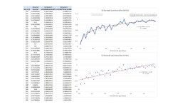
Your x-data cover the interval [154,195], and when your x-y data pairs are selected and a Line chart inserted, Excel will default to creating two curves: 1) one curve of the actual x-data, but treated as though they are y values having assumed x-values of 1, 2, 3,...; and 2) the other curve of the actual y-data, again having assumed x-values of 1, 2, 3, etc. If you then delete the line containing the actual x-values you are left with the actual y-data, and its shape is identical to what you would expect because your actual x-data increases is a sequence increasing by 1 (so there is no stretching or compression of the curve horizontally). Nearly anything can then be specified for the x-axis labels, but the underlying values used by Excel are 1, 2, 3, etc. The actual x-values are irrelevant. Below is an example where I substituted your actual x-values with the Fibonacci sequence (completely non-sensical, but illustrative). The Line chart depiction appears to have the correct shape, but the x-axis labels mean nothing with regard to how regression is handled. I selected the curve and added a logarithm trend line, and the results are the same as what you originally showed. But there is a clue here that helps to arrive at your most recent preferred model form. Note that the trend line appearance is the same as what you wanted. Excel obtained this trend line assuming x-values covering the interval [1,42], so the "x" in the trendline equation -- let's call it x0 -- needs to produce those values when using the actual x-values of [154,195]...therefore x0 = x-153, which leads to your most recent model form: y=0.2222*ln(x-153)+0.1275

 

[stellanhakansson]

Dear Kirk,
Many thanks for you engagement and sharing your Excel wit. I have definitely learned a lot. Problem solved.
All the best,
/Stellan

 

[KRice]

I'm happy to help.