Curve fitting

JenniferMurphy

Well-known Member
Joined
Jul 23, 2011
Messages
2,535
Office Version
  1. 365
Platform
  1. Windows
I have been experimenting with brewing tea at different temperatures. My usual practice is to heat water in a Pyrex in the microwave. By trial and error, I found that it takes about 3-4 minutes to bring 16 oz to a boil. But what if I want water at 180°?

So I took a few readings. Here are the results:

C/R
DEFGH
3TimeWater
Temperature
4(Min)(oz)StartEnd°/min
5
3:00
16
66.7
179.537.6000
62:301670.0168.239.2800
72:001672.0153.740.8500
81:301669.1136.945.2000
91:001666.7
116.449.7000
10
68.9
Average

<tbody>
</tbody>

As expected, the hotter the water gets, the more slowly the temperature increases.

I would like to come up with an equation based on this data that will allow me to calculate how many minutes to set the microwave for to get a specific temperature, like 180°.

The function would need to have a horizontal asymptote at 212°. For my data, it is more like 208°. By the time I get my little digital thermometer in the beaker, it has lost a few degrees.

I can't seem to come up with a way to fit a curve to this data. Can anyone help?

Thanks
 
The coefficients are derived by the fit.

But your coefficients had two decimal places: "-3.406.6" and "1.323.8". What are the correct coefficients?

Have you never plotted data and used the Trend Lines? e.g. Trendline in Excel - EASY Excel Tutorial

As I explained, a two degree polynomial was the best fit.

The best fit to what?

Did you take my 5 data points and add the time=0 data point of the average (68.9)?

Code:
Time  Temp
0.0   68.9
1.0  116.4
1.5  136.9
2.0  153.7
2.5  168.2
3.0  179.5

When I do that, I get this equation:

Code:
y = -3.3380952*x^2 + 47.6809524*x + 67

We are pretty close on A and C, but way off on B.

My equation fits the data pretty well up to time=3.0, but then quickly goes well above 212 at about time=4.5.

Of course when you round the coefficients, you compound error and reduce R^2.

I did not "round" the coefficients. I merely pointed out that they had too many decimal points.

An exponential fit was actually the worst fit but as fits go, I consider any R^2 of 0.90 or better a very good fit. Exponential also had an R^2 of 1. Polynomial fits are easy to determine in VBA.

That plot only applies to your data which assumes certain conditions like your average "room temperature", 68.9F, and the power of your microwave, and volume of water, and your type of water.

No, I don't want to assume specific values for any of those conditions. I am not trying to simulate the heating process. I am trying to fir the data I have which takes into account those conditions.

It is easy enough to solve that equation by the Add-In Solver. I may work up one or more VBA direct solutions if that appeals to you.

I'm not sure what equation you are talking about.

I found some info on equations with asymptotes. I'll play around with them a bit.
 
Upvote 0

Excel Facts

Format cells as date
Select range and press Ctrl+Shift+3 to format cells as date. (Shift 3 is the # sign which sort of looks like a small calendar).
I did not set the 0 data point earlier. My time value was incorrect.

Note that post 11's 1.5 <> 00:01:30. Equations vary depending on the values. 00:01:30 is much less than 1.5. So whichever time value you go with will govern your equation coefficients and the fit.

I corrected my time values to be your mm:ss.

When one adds the 0 point as you did in post 11, log and power fits fail in this case. I do recommend doing the plot method and not rely strictly on an R^2 being the sole reason to pick a fitted trend line equation.

I do recommend when doing an experiment like that to start at the same temperature and make the time and final temperature the ranges to plot. I start at the same temperature by using a waterbath.

For this case, I would just go with a linear equation. Post 1: =TREND(D5:D9,G5:G9,180) = 00:02:55
Post 11: =TREND(D5:D10,G5:G10,180) = 00:02:51

Why did not =Trend not show 00:3:00? That is because it is the last data point so prediction is less accurate.

I could show you how to do the polynomial equation by VBA or equation. Linear regression, (=LinEst), R^2 was 0.9823, Poly2Degree was 0.9895, Poly3Degree was 0.9897. It basically boils down to 0.98 or 0.99. Both are very good fits.

A wood stick in your water might be a good idea as you increase time.
 
Last edited:
Upvote 0
Here is my polynomial solution.
Code:
'=Y1PolyFit(180,D5:D10,G5:G10,2) = 00:02:57
'=Y1PolyFit(180,D5:D10,G5:G10,3) = 00:02:58
Function Y1PolyFit(xVal#, known_ys, known_xs, iDegree&) As Double
  Dim coeffs
  coeffs = PolyFit(known_ys, known_xs, iDegree)
  Y1PolyFit = YPolyFit(xVal, coeffs)
End Function

Function YPolyFit(xVal#, coeffs) As Double
  YPolyFit = WorksheetFunction.SeriesSum(xVal, UBound(coeffs) - 1, -1, coeffs)
End Function

Function PolyFit(known_ys As Variant, known_xs As Variant, iDegree&)
  Dim pf, i&, a()
  ReDim a(1 To iDegree)
  
  For i = 1 To iDegree
    a(i) = i
  Next i
  pf = Application.LinEst(known_ys, Application.Power(known_xs, a()))
  
  PolyFit = pf
End Function
 
Last edited:
Upvote 0
I did not set the 0 data point earlier. My time value was incorrect.

Note that post 11's 1.5 <> 00:01:30. Equations vary depending on the values. 00:01:30 is much less than 1.5. So whichever time value you go with will govern your equation coefficients and the fit.

I don't know you keep time in Tecumseh (I've heard that "Southern" time is somewhat more relaxed), but here 00:01:30 is 1 minute and 30o seconds, which is exactly 1.5 minutes. :confused:

I corrected my time values to be your mm:ss.

When one adds the 0 point as you did in post 11, log and power fits fail in this case. I do recommend doing the plot method and not rely strictly on an R^2 being the sole reason to pick a fitted trend line equation.

I do recommend when doing an experiment like that to start at the same temperature and make the time and final temperature the ranges to plot. I start at the same temperature by using a waterbath.

That's way too much trouble for what I need. Accuracy to 5 seconds (or even 10) is good enough for me.

For this case, I would just go with a linear equation. Post 1: =TREND(D5:D9,G5:G9,180) = 00:02:55
Post 11: =TREND(D5:D10,G5:G10,180) = 00:02:51

Why did not =Trend not show 00:3:00? That is because it is the last data point so prediction is less accurate.

I could show you how to do the polynomial equation by VBA or equation. Linear regression, (=LinEst), R^2 was 0.9823, Poly2Degree was 0.9895, Poly3Degree was 0.9897. It basically boils down to 0.98 or 0.99. Both are very good fits.

I'm not following a lot of what you are doing. We are either on different pages, or you are way over my head.

A wood stick in your water might be a good idea as you increase time.

Really?
 
Upvote 0
Here is my polynomial solution.

How is this better than the least squares polynomial fit you came up with earlier?

Ken,

I really appreciate all the work you have done, but I don't think it's doing what I need or maybe I just don't understand it.

I did a little fiddling around and came up with this equation:

Code:
y = 212 - 143 x e^(-x/2.1)

This fits my data, including the (0,69) data point, about as well as the polynomial equation

Code:
y = -3.3380952*x^2 + 47.6809524*x + 67

and it has a horizontal asymptote at y=212.

But, after thinking about it a little more, I am inclined to agree with Shg. It's not really an asymptote. The water will boil (at whatever temp that is at my altitude). So, the polynomial curve fit is probably best and just limit it to the point where it hits 212.

Again, thanks for all the work you did.
 
Upvote 0
I guess it is "better" since it is easy to use as a UDF and versatile?

If you care to see what I did using my methods and yours see: https://www.dropbox.com/s/js04r9jk3qss7ld/Microwave Water To Temperature.xlsm?dl=0
Sheet2 shows post 15 equations. Note the bias sums. A perfect fit would show bias=0 for all data points which you can see relates to R^2 being 1 for a perfect fit.

Module mMain shows how to use Solver in VBA to solve your exponential equation in Sheet2. The first set of equations for your polynomial, I used solver dialog.

Note that the values shown in a Plots Trend Line equation are usually formatted General. You can change the number format in the Trend Line's Label to say 15 decimal places if you need more accuracy.
 
Upvote 0
Here's another way:

A​
B​
C​
D​
E​
F​
G​
H​
I​
1​
Time [h:m:s]
Vol (oz]
T(start)
T(end)
DT
deg•oz/day
2​
0:01:00​
16​
66.7​
116.4​
49.7​
1,145,088​
E2: =D2-C2
3​
0:01:30​
16​
69.1​
136.9​
67.8​
1,041,408​
F2: =(D2-C2) * B2 / A2
4​
0:02:00​
16​
72.0​
153.7​
81.7​
941,184​
5​
0:02:30​
16​
70.0​
168.2​
98.2​
905,011​
6​
0:03:00​
16​
66.7​
179.5​
112.8​
866,304​
7​
8​
m
b
9​
0.99555​
1405962.2​
E9:F9: {=LOGEST(F2:F6, E2:E6)}

For each data point, calculate the delta T and the deg*oz/day required to effect the change. Fit col F to col E using the exponential regression in E9:F9.

Now plug the input values back in and calculate the time:

A​
B​
C​
D​
E​
F​
G​
H​
I​
11​
Vol (oz]
T(start)
T(end)
DT
deg•oz/day
Time [h:m:s]
12​
16​
66.7​
116.4​
49.7​
1,126,164​
0:01:01​
E12: =D12-C12
13​
16​
69.1​
136.9​
67.8​
1,038,734​
0:01:30​
F12: =$F$9*$E$9^E12
14​
16​
72.0​
153.7​
81.7​
976,227​
0:01:56​
G12: =B12*E12/F12
15​
16​
70.0​
168.2​
98.2​
906,893​
0:02:30​
16​
16​
66.7​
179.5​
112.8​
849,661​
0:03:04​

As shown in col G, they come back pretty close (within a couple of percent).

How well that translates to different volumes and different initial temps is left to the experimenter.
 
Last edited:
Upvote 0
PS: Don't forget to stir the water before measuring the temp.
 
Upvote 0

Forum statistics

Threads
1,215,250
Messages
6,123,887
Members
449,131
Latest member
leobueno

We've detected that you are using an adblocker.

We have a great community of people providing Excel help here, but the hosting costs are enormous. You can help keep this site running by allowing ads on MrExcel.com.
Allow Ads at MrExcel

Which adblocker are you using?

Disable AdBlock

Follow these easy steps to disable AdBlock

1)Click on the icon in the browser’s toolbar.
2)Click on the icon in the browser’s toolbar.
2)Click on the "Pause on this site" option.
Go back

Disable AdBlock Plus

Follow these easy steps to disable AdBlock Plus

1)Click on the icon in the browser’s toolbar.
2)Click on the toggle to disable it for "mrexcel.com".
Go back

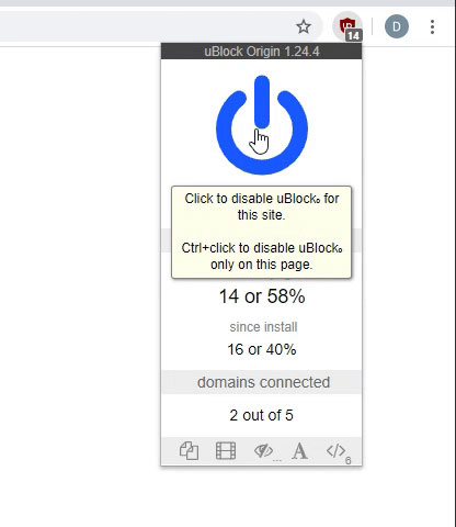
Disable uBlock Origin

Follow these easy steps to disable uBlock Origin

1)Click on the icon in the browser’s toolbar.
2)Click on the "Power" button.
3)Click on the "Refresh" button.
Go back

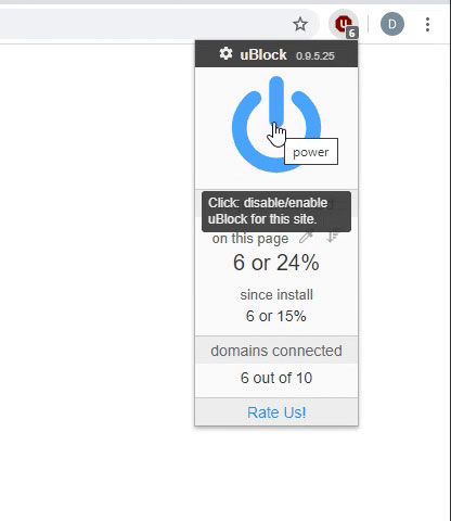
Disable uBlock

Follow these easy steps to disable uBlock

1)Click on the icon in the browser’s toolbar.
2)Click on the "Power" button.
3)Click on the "Refresh" button.
Go back
Back
Top