Data displaying in column instead of row.

[xFrosty]

Hi there,

I have tried using Chat GPT to assist me with this particular thing I'm trying to achieve but I feel that I am entering the same formula over and over again just different ways of entering it in.

So here I am, frustrated because I've spent way too much time trying to get Excel to do what I want it to do.

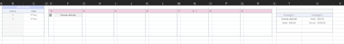
So basically, I am trying to create a calendar thats a set and forget type thing. I have all the data matching to the dates etc, but what I want now is these particular figures to go into another cell(s) so I can track how much from each pay I need to set aside each week. I want the figures to go down the column, so far I've only managed to get them to appear across.

Heres where you come in.... Please help me before I give up! hahahaha.

These are the things I've tried

=IFERROR(INDEX($E$6:$R$10,SMALL(IF(ISNUMBER(SEARCH("S -",$E$6:$R$10)),ROW($E$6:$R$10)-ROW($E$6:$R$10)+1),ROW(INDIRECT("1:"&COUNTIF($E$6:$R$10,"S -*"))))),COLUMN(A1))

This one looked to be wanting to display the text I want but I only have the number 1 showing down the array.

Sample.xlsx
	A	B	C	D	E	F	G	H	I	J	K	L	M	N	O	P	Q	R	S	T
1		November
2	##########
3	##########				Sunday		Monday		Tuesday		Wednesday		Thursday		Friday		Saturday			I want it to display this
4	##########																			S - Phone
5					28		29		30		1		2		3		4			S - Debt
6		` BILL & DEBT PAYMENTS CALENDAR `			S - Phone						S - Debt		S - Power							S - Power
7													S - School							S - School
8		TODAY'S DATE
9		Tuesday, 7 Nov 2023			Don’t want it to display this
10					Found	Not Found	Not Found	Not Found	Not Found	Not Found	Found	Not Found	Found	Not Found	Not Found	Not Found	Not Found	Not Found
11					Not Found	Not Found	Not Found	Not Found	Not Found	Not Found	Not Found	Not Found	Found	Not Found	Not Found	Not Found	Not Found	Not Found
12		MONTH	YEAR		Not Found	Not Found	Not Found	Not Found	Not Found	Not Found	Not Found	Not Found	Not Found	Not Found	Not Found	Not Found	Not Found	Not Found
13		November	2023
14
15		START DAY
16		Monday			1
17					1
18					1
19					1
20
Sheet1

Cell Formulas
Range	Formula
B1	B1	=B13
A2	A2	=DATE(C13,A1,1)
A3	A3	=EOMONTH(A2,0)
A4,B9	A4	=TODAY()
E5	E5	=IF(B16="Sunday", A2 - WEEKDAY(A2, 1) + 1, IF(B16="Monday", A2 - WEEKDAY(A2, 2) + 1, ""))
G5,Q5,O5,M5,K5,I5	G5	=E5 + 1
E10:R12	E10	=IF(ISNUMBER(SEARCH("S -", E6:R8)), "Found", "Not Found")
E16:E19	E16	=IFERROR(INDEX($E$6:$R$8,SMALL(IF(ISNUMBER(SEARCH("S -",$E$6:$R$8)),ROW($E$6:$R$10)-ROW($E$6:$R$10)+1),ROW(INDIRECT("1:"&COUNTIF($E$6:$R$10,"S -*"))))),COLUMN(A1))
Dynamic array formulas.

Cells with Conditional Formatting
Cell	Condition		Cell Format	Stop If True
C13	Cell Value	beginning with "✓"	text	NO
G5	Expression	=G5=TODAY()	text	NO
G5	Expression	=MonthToDisplayNumber<>MONTH(G5)	text	NO
E6:E7	Cell Value	contains "Payday"	text	NO
E6:E7	Expression	=E6=TODAY()	text	NO
E6:E7	Expression	=MonthToDisplayNumber<>MONTH(E6)	text	NO
E8	Cell Value	contains "Payday"	text	NO
E8	Expression	=E8=TODAY()	text	NO
E8	Expression	=MonthToDisplayNumber<>MONTH(E8)	text	NO
F5,H5,J5,L5,N5,P5,R5	Cell Value	contains "Payday"	text	NO
E5	Expression	=E5=TODAY()	text	NO
E5	Expression	=MonthToDisplayNumber<>MONTH(E5)	text	NO
G6:G8,I6:I8,K6:K8,M6:M8,O6:O8,Q6:Q8	Cell Value	contains "Payday"	text	NO
F5,K5:R5,H5:I5,G6:G8,I6:I8,K6:K8,M6:M8,O6:O8,Q6:Q8	Expression	=F5=TODAY()	text	NO
O8	Expression	=MonthToDisplayNumber<>MONTH(O8)	text	NO
F5,K5:R5,O6:O7,K6:K8,H5:I5,I6:I8,G6:G8,M6:M8,Q6:Q8	Expression	=MonthToDisplayNumber<>MONTH(F5)	text	NO

 

[Peter_SSs]

can this be used on different areas, such as E6:R10,E13:R17, E20:J24

Sample data and expected results?

 

[xFrosty]

Sample.xlsx
	D	E	F	G	H	I	J	K	L	M	N	O	P	Q	R	S	T	U
2
3		Sunday		Monday		Tuesday		Wednesday		Thursday		Friday		Saturday
4
5		30		31		1		2		3		4		5			Phone - $34
6		S - Phone - $34						S - Debt - $30		S - Power - $100							Debt - $30
7										S - School - $56							Power - $100
8																	School - $56
9
10
11
12
13																	Total Needed	$ -
14
15
16
17
18
19
20
21
22
23
24
25
26
27
28
29
Sheet1

Cell Formulas
Range	Formula
E5	E5	=IF(B16="Sunday", A2 - WEEKDAY(A2, 1) + 1, IF(B16="Monday", A2 - WEEKDAY(A2, 2) + 1, ""))
G5,Q5,O5,M5,K5,I5	G5	=E5 + 1
T5:T8	T5	=FILTERXML("<p><c>"&SUBSTITUTE(TEXTJOIN("</c><c>",1,E6:R10,E13:R17, E20:J24),"S - ","")&"</c></p>","//c")
U13	U13	=SUM(U5:U12)
Dynamic array formulas.

Cells with Conditional Formatting
Cell	Condition		Cell Format	Stop If True
T5:U8	Cell Value	contains "Payday"	text	NO
T5:U8	Expression	=T5=TODAY()	text	NO
T5:U8	Expression	=MonthToDisplayNumber<>MONTH(T5)	text	NO
G5	Expression	=G5=TODAY()	text	NO
G5	Expression	=MonthToDisplayNumber<>MONTH(G5)	text	NO
E6:E7	Cell Value	contains "Payday"	text	NO
E6:E7	Expression	=E6=TODAY()	text	NO
E6:E7	Expression	=MonthToDisplayNumber<>MONTH(E6)	text	NO
E8	Cell Value	contains "Payday"	text	NO
E8	Expression	=E8=TODAY()	text	NO
E8	Expression	=MonthToDisplayNumber<>MONTH(E8)	text	NO
F5,H5,J5,L5,N5,P5,R5	Cell Value	contains "Payday"	text	NO
E5	Expression	=E5=TODAY()	text	NO
E5	Expression	=MonthToDisplayNumber<>MONTH(E5)	text	NO
G6:G8,I6:I8,K6:K8,M6:M8,O6:O8,Q6:Q8	Cell Value	contains "Payday"	text	NO
F5,K5:R5,H5:I5,G6:G8,I6:I8,K6:K8,M6:M8,O6:O8,Q6:Q8	Expression	=F5=TODAY()	text	NO
O8	Expression	=MonthToDisplayNumber<>MONTH(O8)	text	NO
F5,K5:R5,O6:O7,K6:K8,H5:I5,I6:I8,G6:G8,M6:M8,Q6:Q8	Expression	=MonthToDisplayNumber<>MONTH(F5)	text	NO

 

[Peter_SSs]

That sample data looks no different to the previous. If they are the expected results on the right then we seem to have regressed to an earlier point where Description and amount are no longer in separate columns..
None of this clarifies to me just what you meant by

can this be used on different areas,

 

[xFrosty]

That sample data looks no different to the previous. If they are the expected results on the right then we seem to have regressed to an earlier point where Description and amount are no longer in separate columns..
None of this clarifies to me just what you meant by

No sorry, the array has expended to a fortnightly basis. Im just trying to find another way around this. Stand by

 

[xFrosty]

Lets just leave it as is, seems too complicated. I wanted to have the exsisting formula search within a 2 weekly basis.

I think this is my final thing.... for now haha.

How do I get the formula to find the dollar amounts in the cell and add them into U13.

Also, how do I get it to search for S - but omit J - and vice versa for his bills.

Sample.xlsx
	D	E	F	G	H	I	J	K	L	M	N	O	P	Q	R	S	T	U	V
3		Sunday		Monday		Tuesday		Wednesday		Thursday		Friday		Saturday
4
5		30		31		1		2		3		4		5			Phone - $34
6		S - Phone - $34						S - Debt - $30		S - Power - $100							Debt - $30
7										S - School - $56							Power - $100
8		J - Audible - $14.00															School - $56
9
10
11
12
13																	Total Needed	$220.00
14
15
16																	J - Audible - $14.00
17
18
19
20
21
22
23
24
25																	Total Needed	$ 14.00
26
27
28
Sheet1

Cell Formulas
Range	Formula
E5	E5	=IF(B16="Sunday", A2 - WEEKDAY(A2, 1) + 1, IF(B16="Monday", A2 - WEEKDAY(A2, 2) + 1, ""))
G5,Q5,O5,M5,K5,I5	G5	=E5 + 1
T5:T8	T5	=FILTERXML("<p><c>"&SUBSTITUTE(TEXTJOIN("</c><c>",1,E6:R7),"S - ","")&"</c></p>","//c")
T16	T16	=FILTERXML("<p><c>"&SUBSTITUTE(TEXTJOIN("</c><c>",1,E8:R9),"S - ","")&"</c></p>","//c")
Dynamic array formulas.

Cells with Conditional Formatting
Cell	Condition		Cell Format	Stop If True
T20:T21	Cell Value	contains "Payday"	text	NO
T20:T21	Expression	=T20=TODAY()	text	NO
T20:T21	Expression	=MonthToDisplayNumber<>MONTH(T20)	text	NO
U20	Cell Value	contains "Payday"	text	NO
U20	Expression	=U20=TODAY()	text	NO
U20	Expression	=MonthToDisplayNumber<>MONTH(U20)	text	NO
T8:T9	Cell Value	contains "Payday"	text	NO
T8:T9	Expression	=T8=TODAY()	text	NO
T8:T9	Expression	=MonthToDisplayNumber<>MONTH(T8)	text	NO
T5:U7,U8	Cell Value	contains "Payday"	text	NO
T5:U7,U8	Expression	=T5=TODAY()	text	NO
T5:U7,U8	Expression	=MonthToDisplayNumber<>MONTH(T5)	text	NO
G5	Expression	=G5=TODAY()	text	NO
G5	Expression	=MonthToDisplayNumber<>MONTH(G5)	text	NO
F5,H5,J5,L5,N5,P5,R5	Cell Value	contains "Payday"	text	NO
E5	Expression	=E5=TODAY()	text	NO
E5	Expression	=MonthToDisplayNumber<>MONTH(E5)	text	NO
G6:G8,I6:I8,K6:K8,M6:M8,O6:O8,Q6:Q8,E6,E8,T18:U19,U17,T16:T17	Cell Value	contains "Payday"	text	NO
F5,K5:R5,H5:I5,G6:G8,I6:I8,K6:K8,M6:M8,O6:O8,Q6:Q8,E6,E8,T18:U19,U17,T16:T17	Expression	=E5=TODAY()	text	NO
O8	Expression	=MonthToDisplayNumber<>MONTH(O8)	text	NO
F5,K5:R5,O6:O7,K6:K8,H5:I5,I6:I8,G6:G8,M6:M8,Q6:Q8,E6,E8,T18:U19,U17,T16:T17	Expression	=MonthToDisplayNumber<>MONTH(E5)	text	NO

 

[xFrosty]

Sigh and this last thing too please, on the 17 November, youll see S and J to indicate our paydays.

How would I enter in a check box beside the phone and have it grey out and strikethrough when a bill has been paid? It didnt come up when I entered this mock up.

Im assuming that it would show the same result in the bills panel on the far right?

Sample.xlsx
	A	B	C	D	E	F	G	H	I	J	K	L	M	N	O	P	Q	R	S	T	U	V
1		PAY DATES
2		Name	Date		13		14		15		16		17	S, J	18		19
3		S	17 Nov			Phone - $34.00														Fortnight 1	Fortnight 2
4		J	17 Nov																	Phone - $34.00	Debt - $30.00
5																				Debt - $30.00	Power - $100.00
6
7
8
9
Sheet1

Cell Formulas
Range	Formula
E1	E1	=IFERROR(IF(MATCH($E$12, $C$29:$C$46, 0), ":★ " & INDEX($B$29:$B$46, MATCH($E$12, $C$29:$C$46, 0)) & " ★", ""), "")
G1	G1	=IFERROR(IF(MATCH($G$12, $C$29:$C$46, 0), ":★ " & INDEX($B$29:$B$46, MATCH($G$12, $C$29:$C$46, 0)) & " ★", ""), "")
I1	I1	=IFERROR(IF(MATCH($I$12, $C$29:$C$46, 0), ":★ " & INDEX($B$29:$B$46, MATCH($I$12, $C$29:$C$46, 0)) & " ★", ""), "")
K1	K1	=IFERROR(IF(MATCH($K$12, $C$29:$C$46, 0), ":★ " & INDEX($B$29:$B$46, MATCH($K$12, $C$29:$C$46, 0)) & " ★", ""), "")
M1	M1	=IFERROR(IF(MATCH($M$12, $C$29:$C$46, 0), ":★ " & INDEX($B$29:$B$46, MATCH($M$12, $C$29:$C$46, 0)) & " ★", ""), "")
O1	O1	=IFERROR(IF(MATCH($O$12, $C$29:$C$46, 0), ":★ " & INDEX($B$29:$B$46, MATCH($O$12, $C$29:$C$46, 0)) & " ★", ""), "")
Q1	Q1	=IFERROR(IF(MATCH($Q$12, $C$29:$C$46, 0), ":★ " & INDEX($B$29:$B$46, MATCH($Q$12, $C$29:$C$46, 0)) & " ★", ""), "")

Cells with Conditional Formatting
Cell	Condition		Cell Format	Stop If True
E3:R7,E8	Cell Value	contains "S -"	text	NO
E8	Expression	=MonthToDisplayNumber<>MONTH(E8)	text	NO
E8	Expression	=MonthToDisplayNumber<>MONTH(E8)	text	NO
F2,H2,J2,L2,N2,P2,R2	Cell Value	contains "Payday"	text	NO
E8	Cell Value	contains "Birthday"	text	NO
E2:R2,K3:K7,M3:M7,E3:E8,Q3:Q7,I3:I7,O3:O7,G4:G7	Cell Value	contains "Payday"	text	NO
F2:R2,K3:K7,M3:M7,Q3:Q7,I3:I7,O3:O7,E2:E8,G4:G7	Expression	=E2=TODAY()	text	NO
P2:Q2	Expression	=P2=TODAY()	text	NO
F2:R2,I3:I7,M3:M7,O3:O7,Q3:Q7,K3:K7,E2:E8,G4:G7	Expression	=MonthToDisplayNumber<>MONTH(E2)	text	NO

 

[Peter_SSs]

How do I get the formula to find the dollar amounts in the cell and add them into U13.

Why not split them out to their own column as in post #9 & below?

Also, how do I get it to search for S - but omit J

xFrosty.xlsm
	E	F	G	H	I	J	K	L	M	N	O	P	Q	R	S	T	U
5	30		31		32		33		34		35		36			Phone	34
6	S - Phone - $34						S - Debt - $30		S - Power - $100							Debt	30
7									S - School - $56							Power	100
8	J - Audible - $14.00															School	56
9
10
11
12
13																Total Needed	220
Sheet1

Cell Formulas
Range	Formula
G5,Q5,O5,M5,K5,I5	G5	=E5 + 1
T5:T8	T5	=FILTERXML("<p><c>"&TEXTJOIN("</c><c>",1,IF(LEFT(E6:Q8,1)="S",TRIM(MID(SUBSTITUTE(E6:Q8,"-",REPT(" ",100)),100,100)),""))&"</c></p>","//c")
U5:U8	U5	=FILTERXML("<p><c>"&TEXTJOIN("</c><c>",1,IF(LEFT(E6:Q8,1)="S",TRIM(RIGHT(SUBSTITUTE(E6:Q8,"-",REPT(" ",100)),100)),""))&"</c></p>","//c")
U13	U13	=SUM(U5#)
Dynamic array formulas.

 

[xFrosty]

Oh, because I want it to search in several rows and columns but it seems that formula doesnt work.

 

[xFrosty]

Bump? If anyone has any ideas?