Data validation based on Sheet Name

SuperX7

New Member
Joined
Dec 29, 2017
Messages
10
Hi guys,

Been racking my head and finally have succumbed to making a post, normally I can find / piece together solutions by lots of google and experimenting but I'm throwing in the towel this time.

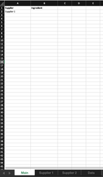
I'm trying to create a sheet where the user selects a supplier in column A (options predetermined by another sheet), and depending on the supplier selected, a list of ingredients is available via a list format data validation in column B.

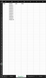
Eg. User selects supplier 1, then the list looks for sheet called "supplier 1" and gives a list of ingredients a user can choose from in Column B (which in screenshot example below is products 1 - 10)

Thanks for your time in looking into this in advance!
 

Attachments

  • Screenshot 2023-12-13 at 18.34.05.png
    Screenshot 2023-12-13 at 18.34.05.png
    24.9 KB · Views: 10
  • Screenshot 2023-12-13 at 18.34.17.png
    Screenshot 2023-12-13 at 18.34.17.png
    30.6 KB · Views: 10

Excel Facts

Lock one reference in a formula
Need 1 part of a formula to always point to the same range? use $ signs: $V$2:$Z$99 will always point to V2:Z99, even after copying
The trick is in the data validation List formula. This assumes the selections in column A of the Main sheet are spelt exactly the same as the sheet names.
Book1
AB
1SupplierIngredient
2Supplier 1
3
Main
Cells with Data Validation
CellAllowCriteria
A2List=$D$1:$D$3
B2List=OFFSET(INDIRECT("'"&A2&"'!B2"),0,0,COUNTA(INDIRECT("'"&A2&"'!B:B"))-1,1)
 
Upvote 0
Solution
Thanks so mich Kevin... that's amazing and works a treat 😀

Would you mind explaining the workings of the formula? Teach a man to fish... as they say
 
Upvote 0
The OFFSET function works like this: OFFSET(<starting point> , <rows from here> , <columns from here> , <height of range in rows> , <width of range in columns>)
For example, this: =OFFSET(A1, 1, 1, 5, 2) would mean starting from cell A1, move down one row and across one column (so you’re now in B2) set the range from this new point to be 5 rows x 2 columns – so you’ve selected the range B2:C6.

The INDIRECT function gives you a reference based on the contents of a cell. So for example, =INDIRECT(A1) would return whatever is in the cell/range that is referred to in cell A1. If cell A1 contained “B50” then the INDIRECT function would return – not what was in cell A1, but what was in cell B50.

The COUNTA function simply counts the number of non-blank cells in the range selected. In the solution, column B (B:B) is referenced – but starting from cell B2, so to exclude B1 from the ‘count’ there is a minus 1 (-1).

References:
OFFSET function - Microsoft Support
INDIRECT function - Microsoft Support
COUNTA function - Microsoft Support.
Thanks! Which part of the formula understands to look within the sheet and not a cell value?
 
Upvote 0

Forum statistics

Threads
1,215,069
Messages
6,122,959
Members
449,096
Latest member
Anshu121

We've detected that you are using an adblocker.

We have a great community of people providing Excel help here, but the hosting costs are enormous. You can help keep this site running by allowing ads on MrExcel.com.
Allow Ads at MrExcel

Which adblocker are you using?

Disable AdBlock

Follow these easy steps to disable AdBlock

1)Click on the icon in the browser’s toolbar.
2)Click on the icon in the browser’s toolbar.
2)Click on the "Pause on this site" option.
Go back

Disable AdBlock Plus

Follow these easy steps to disable AdBlock Plus

1)Click on the icon in the browser’s toolbar.
2)Click on the toggle to disable it for "mrexcel.com".
Go back

Disable uBlock Origin

Follow these easy steps to disable uBlock Origin

1)Click on the icon in the browser’s toolbar.
2)Click on the "Power" button.
3)Click on the "Refresh" button.
Go back

Disable uBlock

Follow these easy steps to disable uBlock

1)Click on the icon in the browser’s toolbar.
2)Click on the "Power" button.
3)Click on the "Refresh" button.
Go back
Back
Top