Divide by VBA

[ashani]

Hi

I wonder if someone could help me with this please.

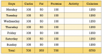
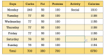
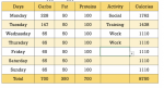
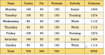
- If in Column G select "social" then increase allowance by 20% of K1 for that particular day
- Also reduced equally for all other days - however the total should remain 700 in Column C.

I'd really appreciate your guidance in the attachment.

thanks

 

[StephenCrump]

Perhaps you can provide some sample results to illustrate?

Otherwise it's not clear which cells are impacted when you say:
- increase allowance?
- reduced equally?

 

[ashani]

Hi
thank you for the message. I have copied 3 examples of the outcome. Hope this is ok.
Many thanks for your help again.

 

[ashani]

Admin - no intention to bring the post up. It’s just another option if I can get any guidance.

Just thinking even if I can get any help with a formula to achieve that if VBA isn’t possible.
thanks

 

[StephenCrump]

This closely replicates your numbers - with some minor rounding differences. We could eliminate the helper cells and combine into one formula, but it would be ugly.

The table at the bottom shows all 8 possibilities assuming SOCIAL days are always in a single block starting on Monday.

	A	B	C	D	E	F	G	H	I	J	K
1											700
2
3			100
4
5			CARBS
6		MON	118				SOCIAL
7		TUE	118				SOCIAL
8		WED	117				SOCIAL
9		THU	117				SOCIAL
10		FRI	77
11		SAT	77
12		SUN	76
13
14
15			Total	Count
16		SOCIAL	470	4
17		NON	230	3
18
19
20		# SOCIAL -->	0	1	2	3	4	5	6	7
21		MON	100	240	159	131	118	110	104	100
22		TUE	100	77	158	131	118	110	104	100
23		WED	100	77	77	131	117	109	104	100
24		THU	100	77	77	77	117	109	104	100
25		FRI	100	77	77	77	77	109	104	100
26		SAT	100	76	76	77	77	77	103	100
27		SUN	100	76	76	76	76	76	77	100
Sheet1

Cell Formulas
Range	Formula
C6:C12	C6	=ROUNDUP(IF(G6="SOCIAL",(C$16-SUMIF(G$5:G5,"SOCIAL",C$5:C5))/(D$16-COUNTIF(G$5:G5,"SOCIAL")),(C$17-SUMIF(G$5:G5,"",C$5:C5))/(D$17+1-COUNTIF(G$6:G6,""))),0)
C16	C16	=7*C$3-ROUND((COUNTBLANK(G$6:G$12))*(6*C3-IF(COUNTIF(G$6:G$12,"SOCIAL"),20%*K$1))/6,0)
D16	D16	=COUNTIF(G$6:G$12,"SOCIAL")
C17	C17	=ROUND((COUNTBLANK(G$6:G$12))*(6*C3-IF(COUNTIF(G$6:G$12,"SOCIAL"),20%*K$1))/6,0)
D17	D17	=COUNTBLANK(G$6:G$12)

 

[ashani]

@StephenCrump
You are an absolute legend and amazing. Thank you so much
Last quick question -
With the same thing - is it possible to have option for "Training" with 10% allowance i.e. From dropdown menu - Social selected than 20% and if Training Selected than 10% otherwise stay as 100 ?

Thank you once again - it's really going to help me with my assignment.

 

[StephenCrump]

... it's really going to help me with my assignment.

Assignment?! What subject are you studying?

So far, I have assumed that the "rule" is:
If any day of the week is SOCIAL, Carbs for each non-SOCIAL day = (700-240)/6 = 76.7 approx.

That doesn't necessarily make sense, but it does replicate your numbers.

Can you explain the "rule" for TRAINING, and illustrate with some examples, including (if this is permitted?) variations with SOCIAL, TRAINING and blank?

 

[StephenCrump]

On looking again, I also realise we can simplify:

C16: =7*C3-H17
C17: =(C3-IF(COUNTIF(G$6:G$12,"SOCIAL"),20%*K1/6))*COUNTBLANK(G$6:G$12)

 

[ashani]

@StephenCrump

Hi Sir,

Thank you once again, honestly I couldn't thank enough for your help. I'm currently studying Maths with actuarial science.
In regards to' Training' so it will work exactly the same way as 'Social' so instead of 'Social' if someones selects Training and the calculation will work on 10% of 700.

If any day of the week is SOCIAL, Carbs for each non-SOCIAL day = (700-240)/6 = 76.7 approx.
If any day of the week is TRAINING, Carbs for each non-TRAINING day = (700-170)/6 = 88.33 approx.

I have attached the example in the sheet - there are 3 options, SOCIAL, TRAINING & WORK. Social will be 20% of 700, Training will be 10% of 700 and Work will remain as whatever the number is- no change.

Once again thank you so much - honestly if you were local I would have brought you something to say thank you

 

[StephenCrump]

I have given you one way to round a total into integer amounts, which in its simplest form is:

	A	B	C	D	E	F	G
1
2
3
4
5
6		MON	118				X
7		TUE	118				X
8		WED	SomethingElse
9		THU	117				X
10		FRI	SomethingElse
11		SAT	117				X
12		SUN	SomethingElse
13
14
15			Total
16		X	470
Sheet1

Cell Formulas
Range	Formula
C6:C12	C6	=IF(G6="X",ROUNDUP((C$16-SUMIF(G$5:G5,"X",C$5:C5))/COUNTIF(G6:G$12,"X"),0),"SomethingElse")

For your assignment, all you need to do is generalise to allow for Y and Z.