Drop down list of users name in columns in order to reference a corresponding cell

[sedwardson]

Hopefully the title isn't too confusing but here is my question. I have a small spreadsheet with users names in columns and then a list of mapped drives above the users names. What I would like to do is have a drop down list (or open to another solution) to select a users name and then in the cell to the right of it, tell me which mapped drives that user is entitled to. The user will only appear once in each column so there shouldn't be any duplicates.

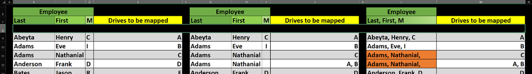
Here is my table to demonstrate what I am trying to achieve (obviously names taken out and replaced for example). I would like to drop down the list of users and select an individual and next to it I would like it to tell me what drive letters (mapped drives) need applying to them.

Drive letters	I	M	H, I, J, K, L	H, J, L		Drop Down List of Users	Drives To Be Mapped
Members	User 1	User 19	User 24	User 29
	User 2	User 20	User 25	User 30
	User 3	User 21	User 26	User 31
	User 4	User 22	User 27
	User 5	User 23	User 28
	User 6
	User 7
	User 8
	User 9
	User 10
	User 11
	User 12
	User 13
	User 14
	User 15
	User 16
	User 17
	User 18

Many thanks for all and any help.

Kind regards

Sam

 

[Fluff]

Another option that removes duplicate drive letters

Fluff.xlsm
	A	B	C	D	E	F	G	H	I	J	K
1	Drive letters	I	M	H, I, J, K, L	H, J, L		Drop Down List of Users	Drives To Be Mapped	OR
2											User 1
3	Members	User 1	User 19	User 24	User 29		User 28	M, H, I, J, K, L			User 2
4		User 2	User 20	User 25	User 30						User 3
5		User 3	User 21	User 26	User 31						User 4
6		User 4	User 22	User 27	User 28						User 5
7		User 5	User 23	User 28							User 6
8		User 6	User 28								User 7
9		User 7									User 8
10		User 8									User 9
11		User 9									User 10
12		User 10									User 11
13		User 11									User 12
14		User 12									User 13
15		User 13									User 14
16		User 14									User 15
17		User 15									User 16
18		User 16									User 17
19		User 17									User 18
20		User 18									User 19
21											User 20
22											User 21
23											User 22
24											User 23
25											User 28
26											User 24
27											User 25
28											User 26
29											User 27
30											User 29
31											User 30
32											User 31
33
Sheet4

Cell Formulas
Range	Formula
K2:K32	K2	=UNIQUE(TOCOL(B3:E100,1,1))
H3	H3	=TEXTJOIN(", ",,UNIQUE(TEXTSPLIT(TEXTJOIN(", ",,FILTER(TOCOL(IF(B3:E100<>"",B1:E1,1/0),2,1),TOCOL(B3:E100,1,1)=G3)),", "),1))
Dynamic array formulas.

Cells with Data Validation
Cell	Allow	Criteria
G3	List	=$K$2#

 

[Royalbloodi]

@Royalbloodi please post all solutions to the board, rather than linking to files as per Rule#4 thanks

Sorry about that.

First off, I've modified a few things and got rid of some useless parts of some formulas.

So, for the Lookup sheet.

What I did was I titled the original sheet 'Lookup Sheet' and then added another named 'Information Sheet'.

On the 'Information Sheet' tab, I created the first set of columns for the First, Last names and Middle Initial as well as a place to input the Drives to be mapped.
There were no formulas for this part.

The second set of columns I created for the purpose of sorting the information. This is done with one formula in the upper right cell that references all the data in the first set and organizes it.

=SORT(B9:E56, 1, 1)

The third set of columns is to merge all the names into individual cells for easy reference with a formula and identify duplicates using Conditional Formatting.

For this one, I used TEXTJOIN to merge the names into one cell each. That formula is:

=TEXTJOIN(", ",TRUE, IF(G9:I9>0,G9:I9," "))

This also removes the commas if the cells are blank.
I then simply referenced the second set of columns to bring over the Drives to be mapped information. I then drag-filled the two separately and selected formatting only.

Finally, to identify duplicate information I used two different Conditional Formatting rules.

The first one is simply applying the Duplicate Rule to the top name in the name column.

Also, to stop this from highlighting the blank cells at the bottom of this column, you include another rule using the Formula to determine cells to format.

The formula for this rule should be =<cell name>="". In this case it is

=L9=""

Now we'll move to setting up the 'Lookup Sheet'.

For this, I made two columns and 25 rows for looking up information.

In the first line for the Employee column, I used Data Validation to set up a drop-down list that references our 'Information Sheet'

At this point, I'll draw your attention to a blank line I colored black on the 'Information Sheet'.

This blank is included in your range for your drop-down list because it makes the list start at the top each time you use it.​

Finally, I put a rather long formula in the top cell of Drives to be mapped. This cell does multiple things.

=IFERROR(INDEX('Information Sheet'!$M$8:$M$81, MATCH(C3, 'Information Sheet'!$L$8:$L$81, 0)),"")

The IFERROR brackets get rid of the N/A if the cell is blank.
The INDEX/MATCH indexes the names and matches the Drives to be mapped to the relative name.

I hope that helps!

 

[Armstrong_N14]

hahaha. i know you've got alot of answers that all works fine, let me make it hard for you by adding another option. LOL..

Book7
	A	B	C	D	E	F	G	H	I	J	K
1	Members	H	I	J	K	L	M	Helper Column		Drop Down List of Users	Drive to be Mapped
2	User 1		1					I		User 31	H
3	User 2		1					I
4	User 3		1					I
5	User 4		1					I
6	User 5		1					I
7	User 6		1					I
8	User 7		1					I
9	User 8		1					I
10	User 9		1					I
11	User 10		1					I
12	User 11		1					I
13	User 12		1					I
14	User 13		1					I
15	User 14		1					I
16	User 15		1					I
17	User 16		1					I
18	User 17		1					I
19	User 18		1					I
20	User 19					1	1	L, M
21	User 20					1	1	L, M
22	User 21					1	1	L, M
23	User 22					1	1	L, M
24	User 23					1	1	L, M
25	User 24	1	1	1	1	1		H, I, J, K, L
26	User 25	1	1	1	1	1		H, I, J, K, L
27	User 26	1	1	1	1	1		H, I, J, K, L
28	User 27	1	1	1	1	1		H, I, J, K, L
29	User 28	1	1	1	1	1		H, I, J, K, L
30	User 29	1						H
31	User 30	1						H
32	User 31	1						H
Sheet1

Cell Formulas
Range	Formula
K2	K2	=VLOOKUP(J2,A:H,8,0)
H2:H32	H2	=TEXTJOIN(", ",,FILTER($B$1:$G$1,(B2:G2=1)))

Cells with Data Validation
Cell	Allow	Criteria
J2	List	=$A$2:$A$32

 

[Armstrong_N14]

t

hahaha. i know you've got alot of answers that all works fine, let me make it hard for you by adding another option. LOL..

Book7
	A	B	C	D	E	F	G	H	I	J	K
1	Members	H	I	J	K	L	M	Helper Column		Drop Down List of Users	Drive to be Mapped
2	User 1		1					I		User 31	H
3	User 2		1					I
4	User 3		1					I
5	User 4		1					I
6	User 5		1					I
7	User 6		1					I
8	User 7		1					I
9	User 8		1					I
10	User 9		1					I
11	User 10		1					I
12	User 11		1					I
13	User 12		1					I
14	User 13		1					I
15	User 14		1					I
16	User 15		1					I
17	User 16		1					I
18	User 17		1					I
19	User 18		1					I
20	User 19					1	1	L, M
21	User 20					1	1	L, M
22	User 21					1	1	L, M
23	User 22					1	1	L, M
24	User 23					1	1	L, M
25	User 24	1	1	1	1	1		H, I, J, K, L
26	User 25	1	1	1	1	1		H, I, J, K, L
27	User 26	1	1	1	1	1		H, I, J, K, L
28	User 27	1	1	1	1	1		H, I, J, K, L
29	User 28	1	1	1	1	1		H, I, J, K, L
30	User 29	1						H
31	User 30	1						H
32	User 31	1						H
Sheet1

Cell Formulas
Range	Formula
K2	K2	=VLOOKUP(J2,A:H,8,0)
H2:H32	H2	=TEXTJOIN(", ",,FILTER($B$1:$G$1,(B2:G2=1)))

Cells with Data Validation
Cell	Allow	Criteria
J2	List	=$A$2:$A$32

this way, whenever you decided to add/delete another drive to be mapped by a user, you will just key in 1 or remove it to their respective column (drive letter)

 

[sedwardson]

Another option that removes duplicate drive letters

Fluff.xlsm
	A	B	C	D	E	F	G	H	I	J	K
1	Drive letters	I	M	H, I, J, K, L	H, J, L		Drop Down List of Users	Drives To Be Mapped	OR
2											User 1
3	Members	User 1	User 19	User 24	User 29		User 28	M, H, I, J, K, L			User 2
4		User 2	User 20	User 25	User 30						User 3
5		User 3	User 21	User 26	User 31						User 4
6		User 4	User 22	User 27	User 28						User 5
7		User 5	User 23	User 28							User 6
8		User 6	User 28								User 7
9		User 7									User 8
10		User 8									User 9
11		User 9									User 10
12		User 10									User 11
13		User 11									User 12
14		User 12									User 13
15		User 13									User 14
16		User 14									User 15
17		User 15									User 16
18		User 16									User 17
19		User 17									User 18
20		User 18									User 19
21											User 20
22											User 21
23											User 22
24											User 23
25											User 28
26											User 24
27											User 25
28											User 26
29											User 27
30											User 29
31											User 30
32											User 31
33
Sheet4

Cell Formulas
Range	Formula
K2:K32	K2	=UNIQUE(TOCOL(B3:E100,1,1))
H3	H3	=TEXTJOIN(", ",,UNIQUE(TEXTSPLIT(TEXTJOIN(", ",,FILTER(TOCOL(IF(B3:E100<>"",B1:E1,1/0),2,1),TOCOL(B3:E100,1,1)=G3)),", "),1))
Dynamic array formulas.

Cells with Data Validation
Cell	Allow	Criteria
G3	List	=$K$2#

Thanks @Fluff , this worked a treat !

 

[Fluff]

You're welcome & thanks for the feedback.

 

[sedwardson]

Another option that removes duplicate drive letters

Fluff.xlsm
	A	B	C	D	E	F	G	H	I	J	K
1	Drive letters	I	M	H, I, J, K, L	H, J, L		Drop Down List of Users	Drives To Be Mapped	OR
2											User 1
3	Members	User 1	User 19	User 24	User 29		User 28	M, H, I, J, K, L			User 2
4		User 2	User 20	User 25	User 30						User 3
5		User 3	User 21	User 26	User 31						User 4
6		User 4	User 22	User 27	User 28						User 5
7		User 5	User 23	User 28							User 6
8		User 6	User 28								User 7
9		User 7									User 8
10		User 8									User 9
11		User 9									User 10
12		User 10									User 11
13		User 11									User 12
14		User 12									User 13
15		User 13									User 14
16		User 14									User 15
17		User 15									User 16
18		User 16									User 17
19		User 17									User 18
20		User 18									User 19
21											User 20
22											User 21
23											User 22
24											User 23
25											User 28
26											User 24
27											User 25
28											User 26
29											User 27
30											User 29
31											User 30
32											User 31
33
Sheet4

Cell Formulas
Range	Formula
K2:K32	K2	=UNIQUE(TOCOL(B3:E100,1,1))
H3	H3	=TEXTJOIN(", ",,UNIQUE(TEXTSPLIT(TEXTJOIN(", ",,FILTER(TOCOL(IF(B3:E100<>"",B1:E1,1/0),2,1),TOCOL(B3:E100,1,1)=G3)),", "),1))
Dynamic array formulas.

Cells with Data Validation
Cell	Allow	Criteria
G3	List	=$K$2#

Hi @Fluff , is there way to list the names in the unique names range in alphabetical order? This is so that when searching in the drop down menu the names appear alphabetically. Thanks again for all your help.

 

[Fluff]

You can use

=sort(UNIQUE(TOCOL(B3:E100,1,1)))

 

[sedwardson]

You can use

=sort(UNIQUE(TOCOL(B3:E100,1,1)))

@Fluff, Thanks, as per usual it work a treat Thank you !

 

[Fluff]

My pleasure.