Drop-down menu entered semi-automatic excel 2019 is it possible?

[AZOUTE]

Hello everyone,

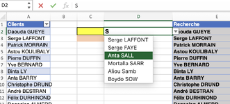
Could I have help: I want to make a drop-down menu with semi-automatic entry but I am blocked by the FILTER function that unfortunately does not exist in Excel 2019 (I am on MAC and using the Excel 2019 version).
I would like to know if by using formulas, we can create an equivalent the FILTER function
Thanks in advance
AZOUTE

Classeur.xlsx
	E
2	#NAME?
Feuil1

Cell Formulas
Range	Formula
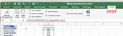
E2	E2	=FILTER(A2:A24,ISNUMBER(SEARCH(C2,A2:A24)),"Pas de résultat")

Cells with Data Validation
Cell	Allow	Criteria
D2	List	=_xlfn.ANCHORARRAY($E$2)
E2	Any value

 

[Peter_SSs]

I adapted your formula like this : =SIERREUR(INDEX(tbl_Clients[#Tout];AGREGAT(15;6;LIGNE(tbl_Clients[Clients])/ESTNUM(CHERCHE(C$2;tbl_Clients[Clients]));LIGNES(E$2:E2)));"")
I got what I was looking for, your help was very precious to me. A big thank you.

You're welcome, but I have some comments.

1. I wonder if you really want the first name returned if C2 is empty like your example above?
   
   
2. That formula is not robust in my view. For example, here it is, working fine

23 10 16.xlsm
	A	B	C	D	E
1	Clients
2	Daouda GUEYE		in		Patrick MORRAIN
3	Serge LAFFONT				Pierre DUFFIN
4	Patrick MORRAIN				Binta LY
5	Astou KOULIBALY				Félix DURHINOND
6	Pierre DUFFIN				Binta TOURE
7	Yve BERNARD				Celestin MAURE
8	Binta LY
9	Anta BARRY
10	Christophe DRUND
11	André BESTRAN
12	Félix DURHINOND
13	Donacien ALMERD
14	Khoudia DIALLO
15	George BRUNDEL
16	Moussa BEYE
17	Alphonse TOURE
18	Oulimata DIAW
19	Astou DIAW
20	Astou FALL
21	Binta TOURE
22	Anta SALL
23	Bruno MENDES
24	Celestin MAURE
25	Braham TALL
26
Filter Replacement (3)

Cell Formulas
Range	Formula
E2:E25	E2	=IF(C$2="","",IFERROR(INDEX(tblClients[#All],AGGREGATE(15,6,ROW(tblClients[Clients])/ISNUMBER(SEARCH(C$2,tblClients[Clients])),ROWS(E$2:E2))),""))

However, if for some reason later any new rows are added at the top of the worksheet, the formulas return incorrect results. Example, if one row is added

23 10 16.xlsm
	A	B	C	D	E
1
2	Clients
3	Daouda GUEYE		in		Astou KOULIBALY
4	Serge LAFFONT				Yve BERNARD
5	Patrick MORRAIN				Anta BARRY
6	Astou KOULIBALY				Donacien ALMERD
7	Pierre DUFFIN				Anta SALL
8	Yve BERNARD				Braham TALL
9	Binta LY
10	Anta BARRY
11	Christophe DRUND
12	André BESTRAN
13	Félix DURHINOND
14	Donacien ALMERD
15	Khoudia DIALLO
16	George BRUNDEL
17	Moussa BEYE
18	Alphonse TOURE
19	Oulimata DIAW
20	Astou DIAW
21	Astou FALL
22	Binta TOURE
23	Anta SALL
24	Bruno MENDES
25	Celestin MAURE
26	Braham TALL
27
Filter Replacement (3)

Cell Formulas
Range	Formula
E3:E26	E3	=IF(C$3="","",IFERROR(INDEX(tblClients[#All],AGGREGATE(15,6,ROW(tblClients[Clients])/ISNUMBER(SEARCH(C$3,tblClients[Clients])),ROWS(E$3:E3))),""))

Points 1 and 2 above could be addressed with these changes to the formula.

23 10 16.xlsm
	A	B	C	D	E
1	Clients
2	Daouda GUEYE		in		Patrick MORRAIN
3	Serge LAFFONT				Pierre DUFFIN
4	Patrick MORRAIN				Binta LY
5	Astou KOULIBALY				Félix DURHINOND
6	Pierre DUFFIN				Binta TOURE
7	Yve BERNARD				Celestin MAURE
8	Binta LY
9	Anta BARRY
10	Christophe DRUND
11	André BESTRAN
12	Félix DURHINOND
13	Donacien ALMERD
14	Khoudia DIALLO
15	George BRUNDEL
16	Moussa BEYE
17	Alphonse TOURE
18	Oulimata DIAW
19	Astou DIAW
20	Astou FALL
21	Binta TOURE
22	Anta SALL
23	Bruno MENDES
24	Celestin MAURE
25	Braham TALL
26
Filter Replacement (3)

Cell Formulas
Range	Formula
E2:E25	E2	=IF(C$2="","",IFERROR(INDEX(tblClients[Clients],AGGREGATE(15,6,(ROW(tblClients[Clients])-ROW(tblClients[#Headers]))/ISNUMBER(SEARCH(C$2,tblClients[Clients])),ROWS(E$2:E2))),""))

Why the formula was not written automatically in cells E3, E4, E5...etc: I would like it to be dynamic

Because Excel 2019 and earlier versions did not support dynamic arrays like MS365 does.

 

[AZOUTE]

=IF(C$3="","",IFERROR(INDEX(tblClients[#All],AGGREGATE(15,6,ROW(tblClients[Clients])/ISNUMBER(SEARCH(C$3,tblClients[Clients])),ROWS(E$3:E3))),""))

Hi, Peter_SSs
Thank you again for your precious remarks: I will take them into account.

In any case, you helped me a lot first, with your formulas but also by allowing me to discover and understand a little the AGGREGATE function.

I wonder if you really want the first name returned if C2 is empty like your example above?

The return of first names (if C2 is empty) gives me the advantage for autocomplete. I created a drop-down menu in cell D2 and slightly modifying your formula by inserting a void between the red quotation marks
=SI(C$3=" ";"";SIERREUR(INDEX(A:A;AGREGAT(15;6;LIGNE(tbl_Clients[Clients])/ESTNUM(CHERCHE(C$3;tbl_Clients[Clients]));LIGNES(E$3:E3)));"")).)

Menuderoulsaisisemiauto.xlsx
	E
2	Daouda GUEYE
Feuil1

Cell Formulas
Range	Formula
E2	E2	=IF(C$3=" ","",IFERROR(INDEX(A:A,AGGREGATE(15,6,ROW(tbl_Clients[Clients])/ISNUMBER(SEARCH(C$3,tbl_Clients[Clients])),ROWS(E$3:E3))),""))

This allows me to make an automatic autocomplete of the surnames and first names in cell D2. (see attached image)

Merci encore pour tout
AZOUTE

 

[AZOUTE]

Because Excel 2019 and earlier versions did not support dynamic arrays like MS365 does.

I asked the question because I noticed that with the SEARCH function, (Excel 2019 does it).
The formula I typed in cell E2 as soon as I validated was automatically written in cells E3, E4, E5,... to E16. You'll notice with me that the formulas in cells E3, E4, E5,... to E16 are grayed out: these are the same effects I wanted to get with this formula:
=SIERREUR(INDEX(tbl_Clients[#Tout];AGREGAT(15;6;LIGNE(tbl_Clients[Clients])/ESTNUM(CHERCHE(C$2;tbl_Clients[Clients]));LIGNES(E$2:E2)));"")

But now I have to do it manually (to copy the formula).

Menuderoulsaisisemiauto.xlsx
	A	B	C	D	E
1	Clientèle
2	Donacien ALMERD		D		TRUE
3	Khoudia DIALLO				TRUE
4	George BRUNDEL				TRUE
5	Moussa BEYE				FALSE
6	Binta LY				FALSE
7	Anta BARRY				FALSE
8	Serge LAFFONT				FALSE
9	Patrick MORRAIN				FALSE
10	Daouda GUEYE				TRUE
11	Pierre DUFFIN				TRUE
12	Yve BERNARD				TRUE
13	Astou KOULIBALY				FALSE
14	Christophe DRUND				TRUE
15	André BESTRAN				TRUE
16	Félix DURHINOND				TRUE
Feuil2

Cell Formulas
Range	Formula
E2:E16	E2	=ISNUMBER(SEARCH(C2,Tab_Clientele[Clientèle]))
Dynamic array formulas.

 

[Peter_SSs]

I do not have Excel 2019 or a Mac to test/check what you are reporting, however a number of things about your results/Excel version(s) are not making much sense to me.

When you select cell E2 in that last sample worksheet, what do you see in the formula bar?
=ISNUMBER(SEARCH(C2,Tab_Clientele[Clientèle]))
or
{=ISNUMBER(SEARCH(C2,Tab_Clientele[Clientèle]))}

I am asking because according to this Microsoft article dynamic array formulas were introduced into Microsoft 365 and may show in older versions as a legacy array formula (one that would have been entered into an older version with Ctrl+Shift+Enter, not just Enter)

Another thing that is not making sense to me is that you say you are using Excel 2019 on a Mac. According to the XL2BB instructions, XL2BB is not compatible with that combination so I'm wondering how you produced that XL2BB Mini Sheet.

 

[AZOUTE]

When you select cell E2 in that last sample worksheet, what do you see in the formula bar?

Here is the answer to this question :
=ESTNUM(CHERCHE(C2;Tab_Clientele[Clientèle]))

NB: I have exactly the same in cells E3, E4, E5,... to E16 but the writings are grayed out

Another thing that is not making sense to me is that you say you are using Excel 2019 on a Mac. According to the XL2BB instructions, XL2BB is not compatible with that combination so I'm wondering how you produced that XL2BB Mini Sheet.

I use Microsoft® Excel for Mac, Version 16.78 (23100802), License: Volume License 2019
See attached image file (Capture d'écran)

According to the XL2BB instructions, XL2BB is not compatible with that combination so I'm wondering how you produced that XL2BB Mini Sheet.

The XL2BB tab, the selection of E2 and the formula in the bar.
See attached image (XL2BB)

Merci
AZOUTE

 

[Peter_SSs]

Thanks for the extra images/information. As I said, I don't have similar hardware or software and was only going on the articles referred to (& I think that I may have mis-interpreted the Microsoft article).
Anyway, if you don't have the 365 functions but do have spill ranges, see what this formula does for you.

AZOUTE.xlsm
	A	B	C	D	E
1	Clients
2	Daouda GUEYE		in		Patrick MORRAIN
3	Serge LAFFONT				Pierre DUFFIN
4	Patrick MORRAIN				Binta LY
5	Astou KOULIBALY				Félix DURHINOND
6	Pierre DUFFIN				Binta TOURE
7	Yve BERNARD				Celestin MAURE
8	Binta LY
9	Anta BARRY
10	Christophe DRUND
11	André BESTRAN
12	Félix DURHINOND
13	Donacien ALMERD
14	Khoudia DIALLO
15	George BRUNDEL
16	Moussa BEYE
17	Alphonse TOURE
18	Oulimata DIAW
19	Astou DIAW
20	Astou FALL
21	Binta TOURE
22	Anta SALL
23	Bruno MENDES
24	Celestin MAURE
25	Braham TALL
26
27
Filter Replacement (3)

Cell Formulas
Range	Formula
E2:E7	E2	=IF(C$2="","",IFERROR(INDEX(tblClients[Clients],AGGREGATE(15,6,(ROW(tblClients[Clients])-ROW(tblClients[#Headers]))/ISNUMBER(SEARCH(C$2,tblClients[Clients])),ROW(INDIRECT("1:"&COUNTIF(tblClients[Clients],"*"&C$2&"*"))))),""))
Dynamic array formulas.

 

[AZOUTE]

As I said, I don't have similar hardware or software

I totally agree with you and I appreciate with great value the help you have given me.

Anyway, if you don't have the 365 functions but do have spill ranges, see what this formula does for you.

=SI(C$2="";"";SIERREUR(INDEX(tbl_Clients[Clients];AGREGAT(15;6;(LIGNE(tbl_Clients[Clients])-LIGNE(tbl_Clients[#Headers]))/ESTNUM(CHERCHE(C$2;tbl_Clients[Clients]));LIGNE(INDIRECT("1:"&NB.SI(tbl_Clients[Clients];"*"&C$2&"*")))));""))

In this formula [#Headers] returns an error. I removed [#Headers] in the formula to eliminate the returned error.

Thus, the formula seems interesting because it pours well into the spill range but it displays in redundancy the value of the first cell of the tbl_Clients table.
Comparing with the old formula in G2, we see that indeed the same amount of cell values returned by the two formulas.

Menuderoulsaisisemiauto.xlsx
	A	B	C	D	E	F	G	H
1	Clients				Recherche
2	Daouda GUEYE		ou		Daouda GUEYE		Daouda GUEYE
3	Serge LAFFONT		ou		Daouda GUEYE		Astou KOULIBALY
4	Patrick MORRAIN				Daouda GUEYE		Khoudia DIALLO
5	Astou KOULIBALY				Daouda GUEYE		Moussa BEYE
6	Pierre DUFFIN				Daouda GUEYE		Alphonse TOURE
7	Yve BERNARD				Daouda GUEYE		Oulimata DIAW
8	Binta LY				Daouda GUEYE		Astou DIAW
9	Anta BARRY				Daouda GUEYE		Astou FALL
10	Christophe DRUND				Daouda GUEYE		Binta TOURE
11	André BESTRAN				Daouda GUEYE		Aliou Samb
12	Félix DURHINOND				Daouda GUEYE		Alioune THIOR
13	Donacien ALMERD
14	Khoudia DIALLO
15	George BRUNDEL
Feuil1

Cell Formulas
Range	Formula
E2:E12	E2	=IF(C$2="","",IFERROR(INDEX(tbl_Clients[Clients],AGGREGATE(15,6,(ROW(tbl_Clients[Clients])-ROW(tbl_Clients))/ISNUMBER(SEARCH(C$2,tbl_Clients[Clients])),ROW(INDIRECT("1:"&COUNTIF(tbl_Clients[Clients],"*"&C$2&"*"))))),""))
G2:G15	G2	=IF(C$3=" ","",IFERROR(INDEX(A:A,AGGREGATE(15,6,ROW(tbl_Clients[Clients])/ISNUMBER(SEARCH(C$3,tbl_Clients[Clients])),ROWS(E$3:E3))),""))
Dynamic array formulas.

Cells with Data Validation
Cell	Allow	Criteria
D2	List	=$E$2:$E$2

 

[Peter_SSs]

I removed [#Headers] in the formula to eliminate the returned error.

Of course removing part of a formula to eliminate an error is more than likely to introduce another error - as it did by not returning the correct results.

I think it is just that you needed to translate #Headers (since it is not an actual column heading) into French. Try this instead

=SI(C$2="";"";SIERREUR(INDEX(tblClients[Clients];AGREGAT(15;6;(LIGNE(tblClients[Clients])-LIGNE(tblClients[#En-têtes]))/ESTNUM(CHERCHE(C$2;tblClients[Clients]));LIGNE(INDIRECT("1:"&NB.SI(tblClients[Clients];"*"&C$2&"*")))));""))

Edit: Oops, I think your table name is actually tbl_Clients

 

[AZOUTE]

Of course removing part of a formula to eliminate an error is more than likely to introduce another error - as it did by not returning the correct results.

Like what it's not always the most the solution

I think it is just that you needed to translate #Headers (since it is not an actual column heading) into French. Try this instead

Indeed, it works 5/5 !
Thank you very much. I'm going to look at the formula to understand it well (you gave me a thread)

Thank you again for your precious help

AZOUTE

 

[AZOUTE]

Like what it's not always the most the solution

OUPS : As it is not always the simplest, the solution

I really appreciated your promptness and efficiency

Thank you very much.
AZOUTE