Duplicate text values in a column

[AFZAL SOHAIL]

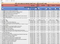
I have data file in which a coloumn c have the following text strings, you see that sr.no.1 & sr.no.13, sr.no.2 and sr.4 are the same, I want to identify through formula the conditional formatting is not working because some are order is not same but they are the same faults, kindly help me

1	8041-GTN to DC-44 Firdous Market
2	FZRD: OLT-1 to C-5 Pak Arab Society
3	8061-ARZ (2/0/7) to C-3/4 Bhobhtian Chowk
4	FRZD: OLT-1 to C-5 Pak Arab Society
5	SMD: MSAG-37 GOR-III to C-32 Cricket House GOR-II & C-3 Rehmania Park
6	C-13 Truck Stand Adda to SMD: OLT-1
7	Bhobhtian Chowk to 8061-ARZ (2/0/7) and C-3/4
8	8061-ARZ (11/0/7) to C-3/4 Bhobtian Chowk Defence Road
9	SMD: OLT-1 to C-13 Truck Stand Adda
10	FZRD: FZRD OLT-1 to MSAG-58 Near Advance Fashion
11	Firdous Market to 8041-GTN DC-44
12	8061-ARZ (2/0/7) to C-3/4 Bhobhtian Chowk Defence Road
13	FZRD: OLT-1 to MSAG-58 near Advance Fashion

 

[AFZAL SOHAIL]

Thanks a lot Sir,
I share the print screen preview before applying conditional formatting of your formula and after applying your formula of conditional formatting.
Sir, I want to know that it is possible to break the cell entry cut into two ends on the basis of " to "" in the cell entry in column-B
and after these two ends results match with colmn-b entry separately

 

[Joe4]

Thanks a lot Sir,
I share the print screen preview before applying conditional formatting of your formula and after applying your formula of conditional formatting.
Sir, I want to know that it is possible to break the cell entry cut into two ends on the basis of " to "" in the cell entry in column-B
and after these two ends results match with colmn-b entry separately

When you are looking for duplicates, are you comparing each value in column A ONLY to the values in column B, or are you also looking for the entry in column A to ALSO match other entries in column A?

 

[Joe4]

I just saw your attachments.
It sounds like you want to insert two columns so you can separate the values in your list, but your AFTER screen print does NOT show that. It only shows Conditional Formatting in place, which is what I already gave you.

So it is still not clear to me what you want, as I already gave you what you are showing in that second screen print.

 

[AFZAL SOHAIL]

Sir,
I want to break the B-col into two pieces on the basis of word "to", i mean break it before word "to",
and after word "to" in cell entry.
And after match these cut pieces of data match with cell entry into Col-B
Thanks a lot too much for your quick response.

 

[Joe4]

OK, then you will need to first insert two blank columns at column C and column D.

Then, enter this formula into cell C6:

=LEFT(B6,FIND(" to ",B6)-1)

and enter this formula in cell D6:

=MID(B6,FIND(" to ",B6)+4,LEN(B6))

and then copy all the way down to the last row with data in column B.

Then, to conditional format/highlight the values in column C which are also found in column D, select the cells starting from cell C6 down to the last cell with values in column C.
Then enter in this Conditional Formatting formula:

=COUNTIF($D:$D,$C6)>0

and select your desired formatting color.

Based on your original data, the results would look like this:

 

[AFZAL SOHAIL]

Sir,
Very very thankful to you, my problems is almost solved,
If you have another trick to solve like these problems kindly share it.
Thanks again Sir,

 

[Joe4]

Very very thankful to you, my problems is almost solved,
If you have another trick to solve like these problems kindly share it.

Is there some part of your question which is still not answered?

The only "trick" is to learn various Excel functions and Conditional Formatting.
The great thing is, most of that can be found on-line rather easily.
For example, if you do a search on "Excel COUNTIF function", you will see many different tutorials, explanations, and examples that show you how to use it.

 

[AFZAL SOHAIL]

Thank you Sir for your advice, my problem is solved but I am only want to know for my knowledge , if I match the col-c or col-d with col-b what will be
the formula for this?
Again thanks Sir,

 

[Joe4]

Thank you Sir for your advice, my problem is solved but I am only want to know for my knowledge , if I match the col-c or col-d with col-b what will be
the formula for this?
Again thanks Sir,

The key is the COUNTIF function, like I showed you in my previous posts:

=COUNTIF($D:$D,$C6)>0

The logic behind it is quite basic. You would use this formula to Conditional Format cell C6.
All that it is saying is to count the number of entries in column D that match the value of cell C6.
If that value is greater than 0 (meaning that there is at least one match), then highlight that cell.

You can use this same function on any cells and columns you want. Just change your ranges to match your needs.

 

[AFZAL SOHAIL]

OK, Thanks a lot Sir: