Duplicates, find values from other columns

[Cervani]

Hi,
I would say this one is tricky (I believe) so I appreciate any comments, including that it's not worthy to even try.

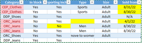
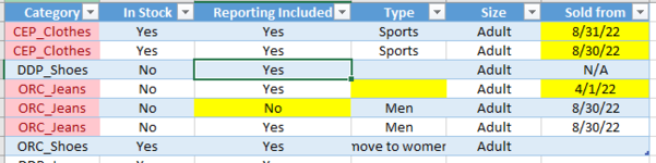
I have an extract in excel - 1k rows, 40 columns. For illustration purpose I will include just 5.

Category column has duplicates as

CEP_Clothes

Sold from values are different

and

ORC_Jeans

Reporting Included , Type , Sold from are different

I highlighted them in yellow.

Category should be distinct, so I need to review all and check why they were duplicated.

Is there is way to do it automatically? Instead of conditional formatting and scrolling to the right, to find different values in other columns?
In other words to have VBA code extracting this to new tab

and this to another

Thanks for any advice.

Table included below.

Category	In Stock	Reporting Included	Type	Size	Sold from
CEP_Clothes	Yes	Yes	Sports	Adult	8/31/22
CEP_Clothes	Yes	Yes	Sports	Adult	8/30/22
DDP_Shoes	No	Yes		Adult	N/A
ORC_Jeans	No	Yes		Adult	4/1/22
ORC_Jeans	No	No	Men	Adult	8/30/22
ORC_Jeans	No	Yes	Men	Adult	8/30/22
ORC_Shoes	Yes	Yes	move to women	Adult
DDP_Jeans	Yes	Yes

 

[Eric W]

With Excel 365, you don't even need VBA. There's a simple formula to do what you want:

Book1
	A	B	C	D	E	F	G	H	I	J	K	L	M	N	O
1	Category	In Stock	Reporting Included	Type	Size	Sold from			Category:		In Stock	Reporting Included	Type	Size	Sold from
2	CEP_Clothes	Yes	Yes	Sports	Adult	8/31/2022			ORC_Jeans	ORC_Jeans	No	Yes	0	Adult	4/1/2022
3	CEP_Clothes	Yes	Yes	Sports	Adult	8/30/2022				ORC_Jeans	No	No	Men	Adult	8/30/2022
4	DDP_Shoes	No	Yes		Adult	N/A				ORC_Jeans	No	Yes	Men	Adult	8/30/2022
5	ORC_Jeans	No	Yes		Adult	4/1/2022
6	ORC_Jeans	No	No	Men	Adult	8/30/2022
7	ORC_Jeans	No	Yes	Men	Adult	8/30/2022
8	ORC_Shoes	Yes	Yes	move to women	Adult
9	DDP_Jeans	Yes	Yes
10
Sheet3

Cell Formulas
Range	Formula
J2:O4	J2	=FILTER(A2:F10,A2:A10=I2)
Dynamic array formulas.

 

[davesexcel]

Not sure what you mean, isn't that what the filters are for?

 

[Cervani]

Doing that manually takes few hrs.

Let's put it this way.
I need to find a reason why category is duplicated.

The reason I have 2x CEP_Clothes is field "Sold from" - there are different values, it's easy to spot on my example.

But what if I have 8 x ORC_Jeans rows, it means that at least 8 columns
have different values ( out of 40 columns)

It's terribly tiring to select first set of duplicates
and look at all columns to find discrepancies . And then next and next. It can be 60 sets of duplicates.

 

[Eric W]

Oh, I see, you only want to show the columns that have differences. Try this:

Book1
	A	B	C	D	E	F	G	H	I	J	K	L
1	Category	In Stock	Reporting Included	Type	Size	Sold from			Category:	Reporting Included	Type	Sold from
2	CEP_Clothes	Yes	Yes	Sports	Adult	8/31/2022			ORC_Jeans	Yes	1/0/1900	4/1/2022
3	CEP_Clothes	Yes	Yes	Sports	Adult	8/30/2022				No	Men	8/30/2022
4	DDP_Shoes	No	Yes		Adult	N/A				Yes	Men	8/30/2022
5	ORC_Jeans	No	Yes		Adult	4/1/2022
6	ORC_Jeans	No	No	Men	Adult	8/30/2022
7	ORC_Jeans	No	Yes	Men	Adult	8/30/2022
8	ORC_Shoes	Yes	Yes	move to women	Adult
9	DDP_Jeans	Yes	Yes
10
Sheet3

Cell Formulas
Range	Formula
J1:L4	J1	=LET(t,FILTER(B1:F10,(A1:A10=I2)+(A1:A10="Category")),r,ROWS(t),tf,t=INDEX(t,2,0),m,MMULT(SEQUENCE(,r,,0),tf+0),FILTER(t,m<r-1))
Dynamic array formulas.

The biggest issue is that I had to format all the columns J:Z (or whatever) as a date format, otherwise you'd just get the number value. This could cause a problem with some other values (like K2 here). But this can be easily remedied with Conditional Formatting. We can set up a rule that looks for certain headings (like "Sold from") and format that with a date, otherwise we'd just leave the standard General format.

 

[Cervani]

Oh, I see, you only want to show the columns that have differences. Try this:

Book1
	A	B	C	D	E	F	G	H	I	J	K	L
1	Category	In Stock	Reporting Included	Type	Size	Sold from			Category:	Reporting Included	Type	Sold from
2	CEP_Clothes	Yes	Yes	Sports	Adult	8/31/2022			ORC_Jeans	Yes	1/0/1900	4/1/2022
3	CEP_Clothes	Yes	Yes	Sports	Adult	8/30/2022				No	Men	8/30/2022
4	DDP_Shoes	No	Yes		Adult	N/A				Yes	Men	8/30/2022
5	ORC_Jeans	No	Yes		Adult	4/1/2022
6	ORC_Jeans	No	No	Men	Adult	8/30/2022
7	ORC_Jeans	No	Yes	Men	Adult	8/30/2022
8	ORC_Shoes	Yes	Yes	move to women	Adult
9	DDP_Jeans	Yes	Yes
10
Sheet3

Cell Formulas
Range	Formula
J1:L4	J1	=LET(t,FILTER(B1:F10,(A1:A10=I2)+(A1:A10="Category")),r,ROWS(t),tf,t=INDEX(t,2,0),m,MMULT(SEQUENCE(,r,,0),tf+0),FILTER(t,m<r-1))
Dynamic array formulas.

The biggest issue is that I had to format all the columns J:Z (or whatever) as a date format, otherwise you'd just get the number value. This could cause a problem with some other values (like K2 here). But this can be easily remedied with Conditional Formatting. We can set up a rule that looks for certain headings (like "Sold from") and format that with a date, otherwise we'd just leave the standard General format.

Thank You Eric, it helps a lot.