Dynamic Index Reference

Kaiser958

New Member
Joined
Jan 19, 2023
Messages
8
Office Version
  1. 2016
Platform
  1. Windows
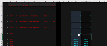
I'm having an issue trying to logic out how to create a looping reference for an INDEX or MATCH formula. What I require is for AR3 and down to represent the index location of S2 and down. I need AR to cycle through that index n number of times where n is the value in the Y column associated the index in Y and then increment into the next index. I can not do this with VBA due to organization restrictions and I really want to keep this with formulas and helper cells, no power query. Any advice is appreciated.
 

Attachments

  • Index Ref.PNG
    Index Ref.PNG
    27.9 KB · Views: 14

Excel Facts

How to create a cell-sized chart?
Tiny charts, called Sparklines, were added to Excel 2010. Look for Sparklines on the Insert tab.
Correction: "...where n is the value in the Y column associated with the index in S and..."
 
Upvote 0
AR2:
Excel Formula:
=IF(COUNTA($AR$1:$AR1)>=SUM($Y$2:$Y$100),"",IFFERROR(IF(COUNTIF($AR$1:$AR1,$AR1)=VLOOKUP($AR1,$S$2:$Y$100,7,0),IFFERROR(INDEX($S$2:$S$100,MATCH(0,INDEX(COUNTIF($AR$1:AR1,$S$2:$S$100),0,0),0)),""),INDEX($S$1:$S$100,ROUNDUP(ROWS($S1:S$2)/VLOOKUP($AR1,$S$2:$Y$100,7,0),0)+1)),$S2))
It's a bit mess but does the job :cool:
Holy hell definitely complex. I'm struggling to implement due to a couple of clerical errors in the translation of my actual product. This has all the components I though I might need but failed to implement. Would you mind walking me through the code as you understand so I can properly install it?
 
Upvote 0
If you share your sample file with first several rows, I can adapt it. It would be easier than explaining 😅 Also I made some typos while I was translating from my native language. I can fix them also.
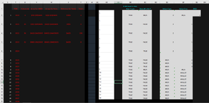
Excel Formula:
=IF(COUNTA($AR$1:$AR1)>=SUM($Y$2:$Y$100),"",IFERROR(IF(COUNTIF($AR$1:$AR1,$AR1)=VLOOKUP($AR1,$S$2:$Y$100,7,0),IFERROR(INDEX($S$2:$S$100,MATCH(0,INDEX(COUNTIF($AR$1:AR1,$S$2:$S$100),0,0),0)),""),INDEX($S$1:$S$100,ROUNDUP(ROWS($S1:S$2)/VLOOKUP($AR1,$S$2:$Y$100,7,0),0)+1)),$S2))
 
Upvote 0
A slightly shorter version:
Excel Formula:
=IF(COUNTA($AR$1:$AR1)<SUM($Y$2:$Y$100),IFERROR(IF(COUNTIF($AR$1:$AR1,$AR1)=VLOOKUP($AR1,$S$2:$Y$100,7,0),IFERROR(INDEX($S$2:$S$100,MATCH($AR1,$S$2:$S$100,-1)+1),""),INDEX($S$1:$S$100,ROUNDUP(ROWS($S1:S$2)/VLOOKUP($AR1,$S$2:$Y$100,7,0),0)+1)),$S2),"")
 
Upvote 0
So using your lastest shortened version, I've installed the code in AR2 and dragged down to 19. The BB Columns and over are the broken down sections of your code to check whats going on. From Row 2 to 8 it works as desired but then completely stops working. I'm sorry, this is the best I can do as far as uploading the sheets. I can't download the minisheet program here at work.

I've labeled the BB and over columns to try to help explain whats going on (with the exception of the iferror checks). I would like to note that my intended use is to start the values in AR3, not AR2. I'm matching the row numbers with the information that will display in the AJ column. I hope this isn't too confusing, I really appreciate the assistance with this.
 

Attachments

  • Index 2.PNG
    Index 2.PNG
    60.1 KB · Views: 7
Upvote 0
To further explain, the information I want as my end goal will go down endlessly in the AJ column. AR will match this since its a 1 for 1 information search function. the S-Y columns are simply index references. They stop in Row 22.
 
Upvote 0
I made it even simpler :) I hope it is more understandable for you:
 
Upvote 0
The numbers in AR10 and down are due to the iferror check returning the $S2 but dragged down to match the row number.
 
Upvote 0

Forum statistics

Threads
1,215,051
Messages
6,122,871
Members
449,097
Latest member
dbomb1414

We've detected that you are using an adblocker.

We have a great community of people providing Excel help here, but the hosting costs are enormous. You can help keep this site running by allowing ads on MrExcel.com.
Allow Ads at MrExcel

Which adblocker are you using?

Disable AdBlock

Follow these easy steps to disable AdBlock

1)Click on the icon in the browser’s toolbar.
2)Click on the icon in the browser’s toolbar.
2)Click on the "Pause on this site" option.
Go back

Disable AdBlock Plus

Follow these easy steps to disable AdBlock Plus

1)Click on the icon in the browser’s toolbar.
2)Click on the toggle to disable it for "mrexcel.com".
Go back

Disable uBlock Origin

Follow these easy steps to disable uBlock Origin

1)Click on the icon in the browser’s toolbar.
2)Click on the "Power" button.
3)Click on the "Refresh" button.
Go back

Disable uBlock

Follow these easy steps to disable uBlock

1)Click on the icon in the browser’s toolbar.
2)Click on the "Power" button.
3)Click on the "Refresh" button.
Go back
Back
Top