Evaluate Pairs: Values in Single Cells

[Pulsar3000]

Hello All:

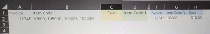
See my picture. Looking for non-VBA solution.

I need to combine Column A with every individual item in Column B (i.e. 12345+10500, 12345+10500A, ect) and if one of these pairs matches the pair in Columns F & G (12345+10500S), then I want the cost put in Column C for the matching pair. In addition, I want the 2nd part of the pair (Item Code 1 = 10500S in this case) that was used to find the cost to be put in Column D.

Although all columns are in one tab in my screenshot, Columns A-D will be in one tab and Columns F-H are in another tab. My real life workbook will have have thousands of rows like shown in Columns A-D and thousands of rows like shown in Columns F-H along with many more columns in each respective tab.

Thank you in advance!

 

[Peter_SSs]

I suggest that you investigate XL2BB for providing sample data to make it easier for helpers by not having to manually type out sample data to test with.

Is this what you mean? If not more varied examples and expected results please.

23 06 23.xlsm
	A	B	C	D	E	F	G	H
1
2	12345	10500, 10500D, 10500S, 10500G	10	10500S		12345	10500S	10
3	12345	10500, 10500D, 10500S, 10500G				12345	10500X	10
4	12345	10500, 10500D, 10500S, 10500G				23456	10500D	10
5	12345	10500, 10500D, 10500S, 10500G	10	10500		12345	10500	10
Match pairs

Cell Formulas
Range	Formula
C2:C5	C2	=IF(AND(F2=A2,ISNUMBER(FIND(" "&G2&","," "&B2&","))),H2,"")
D2:D5	D2	=IF(C2="","",G2)

 

[Pulsar3000]

I suggest that you investigate XL2BB for providing sample data to make it easier for helpers by not having to manually type out sample data to test with.

Is this what you mean? If not more varied examples and expected results please.

23 06 23.xlsm
	A	B	C	D	E	F	G	H
1
2	12345	10500, 10500D, 10500S, 10500G	10	10500S		12345	10500S	10
3	12345	10500, 10500D, 10500S, 10500G				12345	10500X	10
4	12345	10500, 10500D, 10500S, 10500G				23456	10500D	10
5	12345	10500, 10500D, 10500S, 10500G	10	10500		12345	10500	10
Match pairs

Cell Formulas
Range	Formula
C2:C5	C2	=IF(AND(F2=A2,ISNUMBER(FIND(" "&G2&","," "&B2&","))),H2,"")
D2:D5	D2	=IF(C2="","",G2)

Hi Peter:

I wasn't sure if I should use my company computer with XL2BB so I just took a picture. Don't have my PC with me.

Except for one part, your solution is working.

I need to search the pairs in Column A and B in the entire Columns F & G. I can add another column to concatenate Columns F & G so that the formula only searches one column. So the first part of the formula in your cell C2 "F2=AA2" won't work as the data won't be neatly lined up in that way. They'll be tens of thousands of rows similar to Columns F & G on a separate worksheet. Same issue with the formula in D2.

 

[Peter_SSs]

I wasn't sure if I should use my company computer with XL2BB so I just took a picture.

A picture with 1 row of data when you want to compare 1 to many is a bit misleading.

It is not as good as a mini sheet but you can copy/paste (small sections only please) directly from Excel, explain ranges and detail requirements in relation to that.

 

[Pulsar3000]

A picture with 1 row of data when you want to compare 1 to many is a bit misleading.

It is not as good as a mini sheet but you can copy/paste (small sections only please) directly from Excel, explain ranges and detail requirements in relation to that.

Yes, the screenshot itself is misleading. However, in my OP in my last paragraph I explained that there's two sets of data with each having thousands of rows in different worksheets. I had described the requirements when I said the below in italics. Nonetheless, I'll provide more data since visuals are more helpful . Thanks for your patience!

Although all columns are in one tab in my screenshot, Columns A-D will be in one tab and Columns F-H are in another tab. My real life workbook will have have thousands of rows like shown in Columns A-D and thousands of rows like shown in Columns F-H along with many more columns in each respective tab.

 

[Pulsar3000]

I couldn't download XL2BB into my work laptop so here's some more data.
In nutshell, I just wanted the part "F2=C2" in @Peter_SSs formula in his cell C2 to search pairs in a column vs a single cell and the same for formula in his cell D2.

In any event here's a more detailed explanation.

I want the cost in the very last column to be put in the third column and the related item code 1 associated with that cost in the fourth column for the matching pair in in the first two columns.

1. For example, in the first column in the first row there's an item 12345 and in the second column there are four item codes.
2. When the pairs are combined without a delimiter, we get the pairs 1234510500, 1234510500A, 1234510500D, and 1234510500W.
3. I want a formula in the third column to look for these pairs in the second to last column with the purple header, which is simply the values from the preceding two columns without delimiters as shown with the blue and orange values.
4. Once it finds the matching pair 1234510500W, I want the $1,800 cost in third column and 10500W in the fourth column.

Note: The data in the first four columns (i.e. Data Set 1) will be in one worksheet with 10s of thousands of rows and the data in the last four columns (Data Set 2) will be in a different worksheet also with 10s of thousands of rows. Both data sets will each have pairs not found in the other data set.

Item	Item Code 1	Cost	Item Code 1 Found		Item	Item Code 1	Item + Item Code 1	Cost
12345​	10500, 10500A, 10500D, 10500W	$1,800	10500W		09087	598405X	09087598405X	$1,000​
90479​	85068, 85068C, 309578				98734​	79800​	9873479800	$1,100​
40928​	10923C, 10923				001928	69078​	00192869078	$1,200​
37859​	039847, 039847Q, 00123				90479​	85068C	9047985068C	$1,500​
09087	598405, 598405X, 098577				34561​	50968​	3456150968	$1,600​
					12345​	10500W	1234510500W	$1,800​
					23456​	385950​	23456385950	$1,900​
					37859​	00123	3785900123	$2,000​
					69086​	59845​	6908659845	$2,100​
					40928​	10923​	4092810923	$2,300​

 

[Peter_SSs]

Thanks for the extra data and explanation.

Is it possible that there could be more than one match for a row? For example, for your first row on the left, could the 2nd last column (Item + Item Code 1) include, say, 1234510500W and on another row 1234510500A?
If so, could the last column (Cost) hold different values on those two rows? If that is also possible which cost should be returned in column C?

 

[Pulsar3000]

Thanks for the extra data and explanation.

Is it possible that there could be more than one match for a row? For example, for your first row on the left, could the 2nd last column (Item + Item Code 1) include, say, 1234510500W and on another row 1234510500A?
If so, could the last column (Cost) hold different values on those two rows? If that is also possible which cost should be returned in column C?

Sure, no problem.
It can be possible but not sure how often that would happen. In any event, it'd be best to plan for it.

In those cases, I would like all the costs found for the pairs in the same cell. I presume a textjoin/unique/filter type of nested function would handle that.

So for example, if more the other pair 1234510500A was found in another row whose cost was $1,500, then the first cell in the third column with the blue/aqua amount of $1,800 would now be $1,800; $1,500 in the same cell. Is this doable or too overly complicated to do with formulas?

Would there be a performance issue with excel calculating if these formulas were in tens of thousands of rows?

 

[Peter_SSs]

Is this what you mean?

Pulsar3000.xlsm
	A	B	C	D	E	F	G	H	I
1	Item	Item Code 1	Cost	Item Code 1 Found		Item	Item Code 1	Item + Item Code 1	Cost
2	12345	10500, 10500A, 10500D, 10500W	1800	10500W		90479	309578	90479309578	$1,000
3	90479	85068, 85068C, 309578	1000; 1500	309578; 85068C		98734	79800	9873479800	$1,100
4	40928	10923C, 10923	2300	10923		1928	69078	192869078	$1,200
5	37859	039847, 039847Q, 00123	2000	123		90479	85068C	9047985068C	$1,500
6	9087	598405, 598405X, 098577				34561	50968	3456150968	$1,600
7						12345	10500W	1234510500W	$1,800
8						23456	385950	23456385950	$1,900
9						37859	123	3785900123	$2,000
10						69086	59845	6908659845	$2,100
11						40928	10923	4092810923	$2,300
Sheet1

Cell Formulas
Range	Formula
C2:C6	C2	=TEXTJOIN("; ",1,FILTER(I$2:I$20000,ISNUMBER(FIND(H$2:H$20000,A2&SUBSTITUTE(B2,", ",", "&A2))),""))
D2:D6	D2	=TEXTJOIN("; ",1,FILTER(G$2:G$20000,ISNUMBER(FIND(H$2:H$20000,A2&SUBSTITUTE(B2,", ",", "&A2))),""))

Would there be a performance issue with excel calculating if these formulas were in tens of thousands of rows?

You will have to test that.

 

[Pulsar3000]

Is this what you mean?

Pulsar3000.xlsm
	A	B	C	D	E	F	G	H	I
1	Item	Item Code 1	Cost	Item Code 1 Found		Item	Item Code 1	Item + Item Code 1	Cost
2	12345	10500, 10500A, 10500D, 10500W	1800	10500W		90479	309578	90479309578	$1,000
3	90479	85068, 85068C, 309578	1000; 1500	309578; 85068C		98734	79800	9873479800	$1,100
4	40928	10923C, 10923	2300	10923		1928	69078	192869078	$1,200
5	37859	039847, 039847Q, 00123	2000	123		90479	85068C	9047985068C	$1,500
6	9087	598405, 598405X, 098577				34561	50968	3456150968	$1,600
7						12345	10500W	1234510500W	$1,800
8						23456	385950	23456385950	$1,900
9						37859	123	3785900123	$2,000
10						69086	59845	6908659845	$2,100
11						40928	10923	4092810923	$2,300
Sheet1

Cell Formulas
Range	Formula
C2:C6	C2	=TEXTJOIN("; ",1,FILTER(I$2:I$20000,ISNUMBER(FIND(H$2:H$20000,A2&SUBSTITUTE(B2,", ",", "&A2))),""))
D2:D6	D2	=TEXTJOIN("; ",1,FILTER(G$2:G$20000,ISNUMBER(FIND(H$2:H$20000,A2&SUBSTITUTE(B2,", ",", "&A2))),""))

You will have to test that.

Yes, it's working great! Thank you so much!!!
I marked your last post as the solution.

The performance seems fine, if it gets bad I'll figure something else out.