Ever-increasing discount curve

toddbeck

New Member
Joined
Jul 12, 2010
Messages
7
I have a unit list price of $10. At 100,000 units, I want the price to be $2.00.

How can I calculate an ever-increasing discount curve between those two points? I want it to be that the more you buy, the deeper the discount.

My amateur efforts so far result in curves that go negative, so I'm paying the customer to buy my stuff. Also, I don't want the total (units x price) to reach a point where it reverses and starts to go down--meaning you pay less total for 300 units than you would total for 200 units.

Does that make sense? Please help. Thank you!
 
In fact it isn't even certain that I did help ...

The beauty is that you will never know if you helped me, Peter.

That's what I did. My question was similar to another so I leveraged their answer.
.. and it doesn't specifically state that "their answer" was provided by me.
You might be on a fruitless search.
 
Upvote 0

Excel Facts

Which Excel functions can ignore hidden rows?
The SUBTOTAL and AGGREGATE functions ignore hidden rows. AGGREGATE can also exclude error cells and more.
I am entirely aware... but I've been at this for 3 days now, this is the closest I've got to a solution, so ill give it my best shot, I'm sure there's a way to decode that formula.

I'm impressed to see just how pervasive the topic is, and how much its littered with lazy solutions (vlookups or ifs), they work but changing any value results in absolute nightmares, Glenns formula was the perfect solution to the problem, if we could only decode it... haha

Its also not the first time ive run into this problem, its plagued me for years, I've finally decided to make a stand and find a solution that is both easily modifiable and simple (one liner) for everyone to use.
 
Upvote 0
seems @GlennUK is still around, I would love him to poke over here and let us know how in the world he managed that formula, I've seen he's like a magician with formulas but rarely explains how us mortals can edit and change them to make them to do other things haha:ROFLMAO:
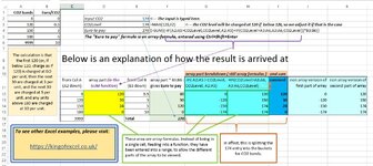
Hi, I am indeed still around - after a long break, when too busy doing paid work. As for how I managed that formula, well, even though it was a long time ago that I first did that logic, I still remember clearly how it hit me ... and I've explained exactly how it works here:
 

Attachments

  • banded_calc.JPG
    banded_calc.JPG
    161.3 KB · Views: 12
Upvote 0
oh thank god you are still here haha, I saw your post, but I think you might be talking about a different formula, this one is the one with the LOG10 function, please for all that is holy tell us how you did it, we have been breaking our heads here for 2 days with no idea how you did it.

The formula in question is this one:
=10-MAX((MIN(LOG10(ROUNDDOWN(K3,IF(K3>100,-2,-(K3>10)))),5)-1)*2,0)
@GlennUK

Basically you managed to integrate the min, max values of the price (10 and 2 dollars) along with the min unit totals (20), set of primary (over 100) and secondary (over 10/20) tiers and steps, along with a lambda value modifier to make it a logarithmic exponential curve, all in that equation... Were stunned, I say we because were a group of 5 people here at the office + 7 more over several forums that just don't know how you did it.
 
Last edited:
Upvote 0
Hi, I am indeed still around - after a long break, when too busy doing paid work. As for how I managed that formula, well, even though it was a long time ago that I first did that logic, I still remember clearly how it hit me ... and I've explained exactly how it works here:
The equation is pure art... all we want is to know how can we change the values

We want to make the prices larger, the min to be 15 instead of 20, be able to adjust the large "step tier" (the 100 one) and be able to adjust the lambda value so we can make the curve(discount) steeper or flatter based on the value entered.
 
Upvote 0
ATM the nearest solution we have found is this, its crude but effective, requires a lot of adjustment but its better than nothing, yours is basically this on steroids:

Thanks to @shg
Diminishing Returns Tests.xlsx
BC
2 First$15.00
3 Last$7.50
4Lambda0.17
5QtyUnit Price
61$15.00
CR1
Cell Formulas
RangeFormula
C6C6=ROUND($C$3+($C$2-$C$3)*(1-$C$4)^(B6-1),2)
 
Upvote 0
well that fizzled fast, this last one works... but runs out of steam around 100-200 units, the price drops so low that its useless.
 
Upvote 0
One way. First is the price for quantity 1, Last is the price for infinite quantity, and k is a factor that controls how fast the price descends from First to Last.


A​
B​
C​
D​
E​
F​
1​
First
10​
2​
Last
5​
3​
k
20​
4​
5​
Qty​
Price​
Total​
Average​
6​
1​
10.00​
10.00​
10.00​
B6: =ExpUnit(A6, First, Last, k)
7​
2​
9.75​
19.75​
9.88​
C6: =ExpTot(A6, First, Last, k)
8​
5​
9.07​
47.62​
9.52​
D6: =C6 / A6
9​
10​
8.15​
90.13​
9.01​
10​
20​
6.89​
164.15​
8.21​
11​
50​
5.40​
342.31​
6.85​
12​
100​
5.03​
599.41​
5.99​

I use some UDFs for this, but you can instead use the formulas shown in the code:

VBA Code:
'============ E x p o n e n t i a l   P r i c i n g   M o d e l ================

' shg 2013, 2021

' Qty   = the number of items
' First = price of the first item
' Last  = price of the last item if you bought an infinite number
' k (1...inf) controls the rate of decrease from First to Last;
' larger decreases slower.

' For large k, k is the qty at which the unit price is
' 1 - 1/e (~63.2%) of the way from First to Last:

'    k     1 - (1 - 1 / k) ^ k
'     2         75.0%
'     5         67.2%
'    10         65.1%
'    20         64.2%
'    50         63.6%
'   100         63.4%

' See MrE552202 - Exponential Pricing.xlsm for additional explanation

Function ExpUnit(Qty As Long, _
                 First As Double, _
                 Last As Double, _
               k As Double) As Double
  ' shg 2013
  ' Returns the incremental price of the Qtyth item

  If k <= 1 Or Qty < 0 Then
    ExpUnit = CVErr(xlErrValue)
  Else
    ExpUnit = (First - Last) * (1 - 1 / k) ^ (Qty - 1) + Last
  End If
End Function

Function ExpTot(Qty As Long, _
                First As Double, _
                Last As Double, _
              k As Double) As Double
  ' shg 2013
  ' Returns the total price for Qty items

  If k < 1 Or Qty < 1 Then
    ExpTot = CVErr(xlErrValue)
  Else
    ExpTot = (First - Last) * (1 - (1 - 1 / k) ^ Qty) * k + Qty * Last
  End If
End Function

Function ExpDisc(Qty As Long, _
                 First As Double, _
                 Last As Double, _
               k As Double) As Variant
  ' shg 2013
  ' Returns the total Discount for Qty items
  ' i.e., Net Price = Qty * First * (1 - ExpDisc(...))

  If Qty <= 0 Then
    ExpDisc = 0
  ElseIf k <= 1 Or Qty < 0 Then
    ExpDisc = CVErr(xlErrValue)
  Else
    'ExpDisc = 1 - (Last / First + (1 - Last / First) * (1 - (1 - 1 / k) ^ Qty) * k / Qty)
    ExpDisc = 1 - ExpTot(Qty, First, Last, k) / (Qty * First)
  End If
End Function

Function ExpDisc2(Qty As Long, _
                  MaxDisc As Double, _
                k As Double) As Variant
  ' shg 2013
  ' Like ExpDisc, but requires only the max discount
  ' i.e., Net Price = Qty * First * (1 - ExpDisc(...))

  If Qty <= 0 Then
    ExpDisc2 = 0
  ElseIf k <= 1 Or Qty < 0 Then
    ExpDisc2 = CVErr(xlErrValue)
  Else
    ExpDisc2 = 1 - ExpTot(Qty, 1, 1 - MaxDisc, k) / Qty
  End If
End Function

Function NetDisc(ListPrice As Double, _
                 DiscZero As Double, _
                 DiscInf As Double, _
               k As Double) As Variant
  ' shg 2013

  ' Returns the Net Discount for ListPrice

  ' Applicable to cases where the discount is based on
  ' total order size rather than item quantity.

  ' DiscZero = Lowest discount (ListPrice = 0)
  ' DiscInf  = Discount for a bazillion dollar order

  ' k = parameter that controls shape
  ' For large k, k is the ListPrice at which discount is 1/e
  ' (~ 36.8%) of the way from DiscZero to DiscInf.

  If k < 1 Then
    NetDisc = CVErr(xlErrNum)
  Else
    If ListPrice <= 0 Then
      NetDisc = DiscZero
    Else
      NetDisc = DiscInf - (DiscInf - DiscZero) * (1 - (1 - 1 / k) ^ ListPrice) * k / ListPrice
    End If
  End If
End Function
 
Upvote 0
I prepared my post before Shg's post.
A clear explanation of your challenge is important,

1. What are you trying to achieve? The following illustrates a tiered approach.
2. You can try a model like the attached and review the arithmetic and the results.
3. You can edit the brackets and/or rates and review the results; see formulas B2 or D2.
4. When you have the brackets and rates that you require, you can name the Bracket information and the Rate differential information.
5. If you define the math that you require, the brackets and rates can be calculated via formula.
Try the formula or formulas that you prefer; formulas D2:E2 require array enter in earlier versions of Excel.
The formulas in C2 and E2 use named arrays. The array of Brackets data and the array of Rate Differentials are named.
See Formulas Name Manger
- The array of Bracket data is named aB Refers to ={0;45000;60000;70000;80000;85000;90000;95000;100000}
- The array of Rate Differentials is named aR Refers to ={10;-1;-1;-1;-1;-1;-1;-1;-1}
Advantages
The formula is easier to read.
The table is not required if the formulas in C2:E2 are used.
N.B.
The names are not necessary; it is a personal preference.
Assign the names to be applicable to the sheet or to the workbook.
Determine the numbers by looking at the tier specifications or by reviewing the ranges.
For example with the formula in B2, select B8:B16-B7:B15 and press F9.

Commission2022.xlsm
ABCDE
1Total Quantity150,000.00
2Price820,000.00820,000.00820,000.00820,000.00
3 " " Arithmetic820,000.00820,000.00820,000.00
4
5
6BracketsRates --- Arithmetic ---
7cell b7 is blankBy BracketCumulative
8010.00300,000.00300,000.00
930,0009.0090,000.00390,000.00
1040,0008.0080,000.00470,000.00
1150,0007.0070,000.00540,000.00
1260,0006.0060,000.00600,000.00
1370,0005.0050,000.00650,000.00
1480,0004.0040,000.00690,000.00
1590,0003.0030,000.00720,000.00
16100,0002.00100,000.00820,000.00
6a
Cell Formulas
RangeFormula
B2B2=SUMPRODUCT(--(B1>A8:A16),B1-A8:A16,B8:B16-B7:B15)
C2C2=SUMPRODUCT(--(B1>aB),B1-aB,aR)
D2D2=SUM((B1>A8:A16)*(B1-A8:A16)*(B8:B16-B7:B15))
E2E2=SUM((B1>aB)*(B1-aB)*aR)
B3B3=D16
C3C3=SUM(C8:C16)
D3D3=(B1>0)*B1*B8+(B1>A9)*(B1-A9)*-1+(B1>A10)*(B1-A10)*-1+(B1>A11)*(B1-A11)*-1+(B1>A12)*(B1-A12)*-1+(B1>A13)*(B1-A13)*-1+(B1>A14)*(B1-A14)*-1+(B1>A15)*(B1-A15)*-1+(B1>A16)*(B1-A16)*-1
C8:C16C8=MAX(0,MIN($B$1,A9)-A8)*B8
D8:D16D8=MAX(0,MIN($B$1,A9)-A8)*B8+N(D7)
 
Upvote 0
The equation is pure art... all we want is to know how can we change the values

We want to make the prices larger, the min to be 15 instead of 20, be able to adjust the large "step tier" (the 100 one) and be able to adjust the lambda value so we can make the curve(discount) steeper or flatter based on the value entered.
Ah, you mean that formula. OK, I'll do some explanations tomorrow, and explain what parts to change for your requirements.
 
Upvote 0

Forum statistics

Threads
1,216,604
Messages
6,131,697
Members
449,666
Latest member
Tommy2Tables365

We've detected that you are using an adblocker.

We have a great community of people providing Excel help here, but the hosting costs are enormous. You can help keep this site running by allowing ads on MrExcel.com.
Allow Ads at MrExcel

Which adblocker are you using?

Disable AdBlock

Follow these easy steps to disable AdBlock

1)Click on the icon in the browser’s toolbar.
2)Click on the icon in the browser’s toolbar.
2)Click on the "Pause on this site" option.
Go back

Disable AdBlock Plus

Follow these easy steps to disable AdBlock Plus

1)Click on the icon in the browser’s toolbar.
2)Click on the toggle to disable it for "mrexcel.com".
Go back

Disable uBlock Origin

Follow these easy steps to disable uBlock Origin

1)Click on the icon in the browser’s toolbar.
2)Click on the "Power" button.
3)Click on the "Refresh" button.
Go back

Disable uBlock

Follow these easy steps to disable uBlock

1)Click on the icon in the browser’s toolbar.
2)Click on the "Power" button.
3)Click on the "Refresh" button.
Go back
Back
Top