excel formula need

[ravindra1962]

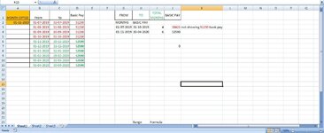
MONTH OPTED	From	to	Basic Pay
Nov-19​	01-07-2019	31-07-2019	51230​
	01-08-2019​	31-08-2019	51230​
	01-09-2019	30-09-2019	51230​
	01-10-2019​	31-10-2019	51230​
	01-11-2019​	30-11-2019	52590​
	01-12-2019​	31-12-2019	52590​
	01-01-2020​	31-01-2020	52590​
	01-02-2020​	29-02-2020	52590​
	01-03-2020​	31-03-2020	52590​
	01-04-2020​	30-04-2020	52590​
IF I HAVE OPTED FOR NOVEMBER 2019
FROM	TO	TOTAL MONTHS	BASIC PAY
01.07.2019	31.10.2019	4 MONTHS	51230​
01.11.2019	30.04.2019	6 MONTHS	52590​
I NEED FORMULA IN EXCEL IN THE ABOVE COLUMNS PLEASE

 

[Toadstool]

Hi Ravindra1962

Your To range of "30.04.2019" appears to be a typo.

Excel will not handle partial date entries so if you type "NOV-19" into a cell it will interpret that incorrectly, e.g. as 19 November 2021. You could force entry as a text field and then use a formula to build a date, but it would be easiest if you just entered the date of the 1st day of the month and year you want to check.

You don't say how the Basic Pay in your results should be calculated so I've assumed it's an average.

I note all ranges are single and complete months and so the formula assumes same.

Ravindra1962.xlsx
	A	B	C	D	E	F	G	H	I	J
1	MONTH OPTED	From	to	Basic Pay			FROM	TO	TOTAL MONTHS	BASIC PAY
2	01-Nov-19	01-Jul-19	31-Jul-19	51230			MONTHS	BASIC PAY
3		01-Aug-19	31-Aug-19	51230			01-Jul-19	31-Oct-19	4	51230
4		01-Sep-19	30-Sep-19	51230			01-Nov-19	30-Apr-20	6	52590
5		01-Oct-19	31-Oct-19	51230
6		01-Nov-19	30-Nov-19	52590
7		01-Dec-19	31-Dec-19	52590
8		01-Jan-20	31-Jan-20	52590
9		01-Feb-20	29-Feb-20	52590
10		01-Mar-20	31-Mar-20	52590
11		01-Apr-20	30-Apr-20	52590
Sheet1

Cell Formulas
Range	Formula
G3	G3	=MIN($B$2:$B$9999)
H3	H3	=A2-1
I3	I3	=COUNTIF($B$2:$B$9999,"<"&$A$2)
J3	J3	=SUMIFS($D$2:$D$9999,$D$2:$D$9999,">0",$B$2:$B$9999,"<"&$A$2)/I3
G4	G4	=A2
H4	H4	=MAX($C$2:$C$9999)
I4	I4	=COUNTIF($B$2:$B$9999,">="&$A$2)
J4	J4	=SUMIFS($D$2:$D$9999,$D$2:$D$9999,">0",$B$2:$B$9999,">="&$A$2)/I4

 

[ravindra1962]

COLUMN J3 SHOWS WRONGLY INSTEAD OF 51230

 

[ravindra1962]

COLUMN J3 SHOWS WRONGLY INSTEAD OF 51230

 

[Toadstool]

You need to start from row D2 and B2. I believe you are starting from D3 and B3.

 

[ravindra1962]

You need to start from row D2 and B2. I believe you are starting from D3 and B3.

I AM STARTING ROW D2 AND B2 THE FORMULA IS

SUMIFS($D$2:$D$11,$D$2:$D$11,">0",$B$2:$B$11,"<"&$A$2)/I3

 

[Toadstool]

Then I suspect one of the date or pay fields is text instead on numeric.

 

[ravindra1962]

Then I suspect one of the date or pay fields is text instead on numeric.

ALL ARE IN NUMERIC

 

[ravindra1962]

DATE FIELD IN DATE FORMAT AND PAY FIELD IS IN NUMERIC

 

[ravindra1962]

IT SHOWS THE CALCULATION LIKE THIS

51230-51230/4=38423