Excel VBA filter ID's on most recent update

[MichaelJ2600]

Hello all

This is a continuation of :

vba code for filtering by latest date

Hey guys, I'm new to the VBA code thing...still in the record macro stage!! I need assistance. I have a worksheet that contains 6 columns, A: Section B: Machine C: Component D: Severity E: Comment F: Date. Now I need a VBA code to filter by the latest date.:confused::confused:

www.mrexcel.com

As I believe I have the same need, but can't get the solution to work. There was a text advising me to create a new post, as the referred was very old, so not trying to be annoying by raising a new thread.

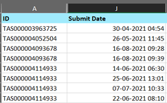
I simply can't get this solution to work. I believe that I have the same setup and requirements as in post #7, however my dates are in column J (10). What I don't understand is, how this filter will look at the Component names in post #7 example, and then filter for the most recent update date in column F (6).

What I want to achieve is one line with the most recent update for each Task ID (column A).

My data:

My target :

My code:

Dim myDate As Date: myDate = Application.Max(Columns(10))
Columns(10).AutoFilter Field:=1, Criteria1:="=" & Format(myDate, [J2].NumberFormat)

I really appreciate any help as I'm stuck.

Thanks
Michael

 

[lrobbo314]

Here is one way.

Book1
	A	B	C	D	E
1	ID	Submit Date		ID	Date
2	TAS000003963725	4/30/2021 4:54		TAS000003963725	4/30/2021 4:54
3	TAS000004052504	5/26/2021 11:45		TAS000004052504	5/26/2021 11:45
4	TAS000004093678	8/16/2021 9:28		TAS000004093678	8/16/2021 9:39
5	TAS000004093678	8/16/2021 9:39		TAS000004114933	7/7/2021 10:33
6	TAS000004114933	6/14/2021 6:30
7	TAS000004114933	6/25/2021 1:01
8	TAS000004114933	7/7/2021 10:33
9	TAS000004114933	6/22/2021 8:10
Sheet3

Cell Formulas
Range	Formula
D2:E5	D2	=LET(id,A2:A9,sd,B2:B9,u,UNIQUE(id),HSTACK(u,MAXIFS(sd,id,u)))
Dynamic array formulas.

 

[MichaelJ2600]

Here is one way.

Book1
	A	B	C	D	E
1	ID	Submit Date		ID	Date
2	TAS000003963725	4/30/2021 4:54		TAS000003963725	4/30/2021 4:54
3	TAS000004052504	5/26/2021 11:45		TAS000004052504	5/26/2021 11:45
4	TAS000004093678	8/16/2021 9:28		TAS000004093678	8/16/2021 9:39
5	TAS000004093678	8/16/2021 9:39		TAS000004114933	7/7/2021 10:33
6	TAS000004114933	6/14/2021 6:30
7	TAS000004114933	6/25/2021 1:01
8	TAS000004114933	7/7/2021 10:33
9	TAS000004114933	6/22/2021 8:10
Sheet3

Cell Formulas
Range	Formula
D2:E5	D2	=LET(id,A2:A9,sd,B2:B9,u,UNIQUE(id),HSTACK(u,MAXIFS(sd,id,u)))
Dynamic array formulas.

Oh, I'm sorry if I was not clear. I'm trying to solve this in a VBA macro, with the purpose to import the result to a new sheet.

/Michael

 

[lrobbo314]

How about this? I have it outputting to range D2. You can change that line for wherever you want the results.

Sub MJ()
Dim AR() As Variant:        AR = Range("A2:B" & Range("A" & Rows.Count).End(xlUp).Row).Value2
Dim SD As Object:           Set SD = CreateObject("Scripting.Dictionary")

For i = 1 To UBound(AR)
    If SD(AR(i, 1)) < AR(i, 2) Then SD(AR(i, 1)) = AR(i, 2)
Next i

With Range("D2").Resize(SD.Count)
    .Value = Application.Transpose(SD.keys())
    .Offset(, 1).Value = Application.Transpose(SD.items())
End With
End Sub

 

[MichaelJ2600]

Hello Irobbo314

I really appreciate your help, but couldn't get it to work, so took the road down to Power BI instead, where I'm, more comfortable. Thanks again, for express-help and focus. Appreciated !