Extract Specific Character Formats from a Text String

[Excel2021]

Hello,

I am trying to extract anything that comes after a hypen and has the following format character format "A123" from a Text String in power query (an excel formula would also work). Occasionally some of the formats I need to pull may vary and contain the format "AA123" or "AA123-AA".

String examples of each type are below in quotes and what I would like to pull is after the = on the right of the strings.

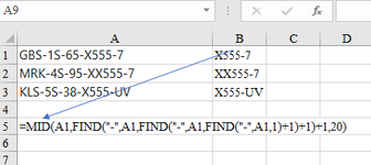
"GBS-1S-65-X555-7" = X555
"MRK-4S-95-XX555-7" = XX555
"KLS-5S-38-X555-UV" = X555-UV

Thanks in Advance.

 

[GraH]

Second try, now I (maybe) understand the query

let
    Source = Excel.CurrentWorkbook(){[Name="Table1"]}[Content],
    #"Changed Type" = Table.TransformColumnTypes(Source,{{"Column1", type text}}),
    #"Added Custom" = Table.AddColumn(#"Changed Type", "Custom", each Text.Combine(List.Select(List.LastN(Text.Split([Column1],"-"),2), each (try Number.FromText(_) otherwise  true) = true),"-"))
in
    #"Added Custom"

Book1
	B	C	D	E	F	G	H	I	J	K	L
1				Column1				Column1	Custom
2				GBS-1S-65-X555-7				GBS-1S-65-X555-7	X555
3				MRK-4S-95-XX555-7				MRK-4S-95-XX555-7	XX555
4				KLS-5S-38-X555-UV				KLS-5S-38-X555-UV	X555-UV
5				KLS-5S-38-X555				KLS-5S-38-X555	X555
6				KLS-5S-38-UV-X555				KLS-5S-38-UV-X555	UV-X555
7
8
9
Sheet1

 

[MOHAMMED A. WASEEM]

Hi
An excel worksheet solution for above.
=MID(A1,FIND("-",A1,FIND("-",A1,FIND("-",A1,1)+1)+1)+1,20)
Thanks
Waseem

 

[GraH]

Hi
An excel worksheet solution for above.
=MID(A1,FIND("-",A1,FIND("-",A1,FIND("-",A1,1)+1)+1)+1,20)
Thanks
Waseem

That's not what the OP described as correct in #7: B1 result should be X555 only, hence not including "-7" in the string.

 

[MOHAMMED A. WASEEM]

Hi
I correct myself. This worksheet formula would do :
=MID(A1,D1+1,FIND("-",A1,FIND("-",A1,FIND("-",A1,FIND("-",A1,1)+1)+1)+1)-1-FIND("-",A1,FIND("-",A1,FIND("-",A1,1)+1)+1))
Thanks

 

[GraH]

Hi
I correct myself. This worksheet formula would do :
=MID(A1,D1+1,FIND("-",A1,FIND("-",A1,FIND("-",A1,FIND("-",A1,1)+1)+1)+1)-1-FIND("-",A1,FIND("-",A1,FIND("-",A1,1)+1)+1))
Thanks

Hi Waseem,

What's in D1 in your solution?
Please use XL2BB code (download link in my signature), so we see the sample data and any parameters you've defined inside cells.
Simply using your formula, returns very odd results.

Book1
	C	D	E	F	G	H
1		Column1	Custom
2		GBS-1S-65-X555-7	X555	X555-7	GBS-
3		MRK-4S-95-XX555-7	XX555	XX555-7	MRK-4
4		KLS-5S-38-X555-UV	X555-UV	X555-UV	KLS-
5		KLS-5S-38-X555	X555	X555	#VALUE!
6		KLS-5S-38-UV-X555	UV-X555	UV-X555	KL
7
Sheet1

Cell Formulas
Range	Formula
F2:F6	F2	=MID(D2,FIND("-",D2,FIND("-",D2,FIND("-",D2,1)+1)+1)+1,20)
G2:G6	G2	=MID(D2,C2+1,FIND("-",D2,FIND("-",D2,FIND("-",D2,FIND("-",D2,1)+1)+1)+1)-1-FIND("-",D2,FIND("-",D2,FIND("-",D2,1)+1)+1))

 

[MOHAMMED A. WASEEM]

Hi
Please find below :
=MID(A1,FIND("-",A1,FIND("-",A1,FIND("-",A1,1)+1)+1)+1,FIND("-",A1,FIND("-",A1,FIND("-",A1,FIND("-",A1,1)+1)+1)+1)-1-FIND("-",A1,FIND("-",A1,FIND("-",A1,1)+1)+1))
Thanks

 

[Excel2021]

Second try, now I (maybe) understand the query

let
    Source = Excel.CurrentWorkbook(){[Name="Table1"]}[Content],
    #"Changed Type" = Table.TransformColumnTypes(Source,{{"Column1", type text}}),
    #"Added Custom" = Table.AddColumn(#"Changed Type", "Custom", each Text.Combine(List.Select(List.LastN(Text.Split([Column1],"-"),2), each (try Number.FromText(_) otherwise  true) = true),"-"))
in
    #"Added Custom"

Book1
	B	C	D	E	F	G	H	I	J	K	L
1				Column1				Column1	Custom
2				GBS-1S-65-X555-7				GBS-1S-65-X555-7	X555
3				MRK-4S-95-XX555-7				MRK-4S-95-XX555-7	XX555
4				KLS-5S-38-X555-UV				KLS-5S-38-X555-UV	X555-UV
5				KLS-5S-38-X555				KLS-5S-38-X555	X555
6				KLS-5S-38-UV-X555				KLS-5S-38-UV-X555	UV-X555
7
8
9
Sheet1

Sorry, I was tied up with other things the past few days. I tried this however I am getting a similar issue where it will only take the UV for some of the strings and ignore the rest.

 

[Excel2021]

Hi
Please find below :
=MID(A1,FIND("-",A1,FIND("-",A1,FIND("-",A1,1)+1)+1)+1,FIND("-",A1,FIND("-",A1,FIND("-",A1,FIND("-",A1,1)+1)+1)+1)-1-FIND("-",A1,FIND("-",A1,FIND("-",A1,1)+1)+1))

Hi
Please find below :
=MID(A1,FIND("-",A1,FIND("-",A1,FIND("-",A1,1)+1)+1)+1,FIND("-",A1,FIND("-",A1,FIND("-",A1,FIND("-",A1,1)+1)+1)+1)-1-FIND("-",A1,FIND("-",A1,FIND("-",A1,1)+1)+1))
Thanks

Hi,

I tried this but I am getting similar results to the power query ones where it seems to have issues with the "UV" parts. I will post a better list of strings. Maybe I am missing some variations.

 

[JEC]

Like I said before, if you want better solutions you have to post more examples with desired outcomes