Extracting text from non-blank cells in a row

nukeemaway

New Member
Joined
Jul 12, 2009
Messages
34
I have a spreadsheet with about 2000 rows and columns from C to AQ, starting at row 6. However, there are numerous blank cells interspersed throughout the sheet at different non-uniform points. I need a formula to extract the text from the non-blank cells so that there are no gaps. On a new sheet would be preferable, but if it can only be done on the same sheet, that is fine.

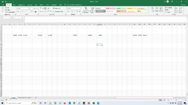
For example, let's say C6, D6, E6, and F6 have text. Then G6 and H6 are blank. Then I6 and J6 have text. Then K6 is blank. Etc.

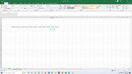
I want to pull all the text so that (preferably on a new sheet), I have the text from C6, D6, E6, F6, I6, and J6 consecutively one after another with no blank cells in between

Thank you so much in advance for the help!

(P.S. I have found solutions on other sites using arrays in various formulas, but none of them seem to be working, as they either pull some blanks or don't pull all of the non-blank cells when I then copy the formula across all the other cells).
 

Excel Facts

Using Function Arguments with nested formulas
If writing INDEX in Func. Arguments, type MATCH(. Use the mouse to click inside MATCH in the formula bar. Dialog switches to MATCH.
Without a sample to test, I think that this may be a way to do it. Load your data into Power Query/Get and Transform found on the Data Tab of the Ribbon. Unpivot your data. Filter out the null rows. Repivot your data. This is a simplistic concept overview without seeing sample data which may change the specific steps.
 
Upvote 0
Here's a macro that will remove the blank cells (if they are truly blank) after the original data sheet is copied to a new sheet named "New Sheet".
VBA Code:
Sub Consolidate()
'run this from the original data sheet
Dim R As Range
ActiveSheet.Copy after:=ActiveSheet
Application.DisplayAlerts = False
On Error Resume Next
Worksheets("New Sheet").Delete
On Error GoTo 0
With ActiveSheet
    .Name = "New Sheet"
    Set R = .Range("C6:AQ" & .Cells(Rows.Count, "C").End(xlUp).Row)
End With
On Error Resume Next
R.SpecialCells(xlCellTypeBlanks).Delete shift:=xlToLeft
On Error GoTo 0
End Sub
 
Upvote 0
Thank you very much. I'm actually trying to look for a non-VBA solution.

These are what I found on other sites (which obviously were tailored for those spreadsheets, which is where I am having difficulty in adapting them:

Either:
1) =IFERROR(INDEX(INDEX($A1:$G1,1,AGGREGATE(15,6,1/(LEN($A1:$G1)>0)*COLUMN($A1:H$1),COLUMN(INDEX($1:$1,1):INDEX($1:$1,COUNTA($A1:$G1))))),COLUMNS($A:A)),"")
or
2) =IF(COLUMNS($A1:A1)>COUNTA($A1:$Z1),"",INDEX($A1:$Z1,SMALL(IF($A1:$Z1<>"",COLUMN($A1:$Z1)),COLUMNS($A1:A1))))

I think #2 requires a ctrl+shift+enter, whereas number 1 does not.

Just for clarity, I'm trying to have a formula on a new sheet so that I can automatically get Sample2 from Sample1.
 

Attachments

  • Sample1.png
    Sample1.png
    135.4 KB · Views: 89
  • Sample2.png
    Sample2.png
    118.6 KB · Views: 88
Upvote 0
Your sample looks like you start in C7, but your OP indicates C6. Assuming its C6 try this:
In C6 on your New Sheet Enter this.
Excel Formula:
=IFERROR(INDEX('Original'!$C6:$AQ6,AGGREGATE(15,6,(COLUMN($C6:$AQ6)-COLUMN($C6)+1)/('Original'!$C6:$AQ6<>""),COLUMNS($C$6:C6))),"")
then drag across to AQ6 and then drag the C6:AQ6 down to cover the data on sheet "Original".
If you want to start at C7 obviously change the C6 to C7 throughout the formula.
 
Upvote 0
Cannot manipulate data in a picture. If you require further assistance, suggest you upload a sample of your data using XL2BB so we don't have to try and replicate what you have and guess at the structure.
 
Upvote 0

Forum statistics

Threads
1,215,064
Messages
6,122,941
Members
449,094
Latest member
teemeren

We've detected that you are using an adblocker.

We have a great community of people providing Excel help here, but the hosting costs are enormous. You can help keep this site running by allowing ads on MrExcel.com.
Allow Ads at MrExcel

Which adblocker are you using?

Disable AdBlock

Follow these easy steps to disable AdBlock

1)Click on the icon in the browser’s toolbar.
2)Click on the icon in the browser’s toolbar.
2)Click on the "Pause on this site" option.
Go back

Disable AdBlock Plus

Follow these easy steps to disable AdBlock Plus

1)Click on the icon in the browser’s toolbar.
2)Click on the toggle to disable it for "mrexcel.com".
Go back

Disable uBlock Origin

Follow these easy steps to disable uBlock Origin

1)Click on the icon in the browser’s toolbar.
2)Click on the "Power" button.
3)Click on the "Refresh" button.
Go back

Disable uBlock

Follow these easy steps to disable uBlock

1)Click on the icon in the browser’s toolbar.
2)Click on the "Power" button.
3)Click on the "Refresh" button.
Go back
Back
Top