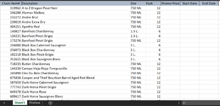
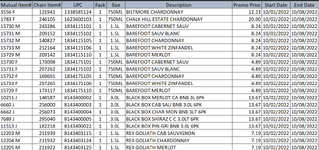
I really need help. I have been trying to figure this out for weeks now. I have a spreadsheet that has UPC numbers and multiple costs with dates. I aim to return the lowest promo price and dates for the Chain Item#.
MrExcelPlayground11.xlsx | |||||||||||||||
---|---|---|---|---|---|---|---|---|---|---|---|---|---|---|---|
A | B | C | D | E | F | G | H | I | J | K | L | M | |||
1 | Best Promo Price and Date Range | Chain Item# | Promo Price | Start Date | End Date | ||||||||||
2 | Chain Item# | Description | Size | Pack | Promo Price | Start Date | End Date | 1 | $15.20 | 10/1/2021 | 10/8/2021 | ||||
3 | 1 | A | 750ml | 12 | $15.20 | 10/1/2021 | 10/8/2021 | 2 | $16.50 | 10/1/2021 | 10/8/2021 | ||||
4 | 2 | B | 750ml | 12 | $16.50 | 10/1/2021 | 10/8/2021 | 3 | $17.80 | 11/1/2021 | 11/8/2021 | ||||
5 | 3 | C | 750ml | 12 | $17.80 | 11/1/2021 | 11/8/2021 | 4 | $19.10 | 12/2/2021 | 12/9/2021 | ||||
6 | 4 | D | 750ml | 12 | $19.10 | 12/2/2021 | 12/9/2021 | 5 | $20.40 | 1/2/2022 | 1/9/2022 | ||||
7 | 5 | E | 750ml | 6 | $20.40 | 1/2/2022 | 1/9/2022 | 6 | $21.70 | 1/2/2022 | 1/9/2022 | ||||
8 | 6 | F | 750ml | 6 | $21.70 | 1/2/2022 | 1/9/2022 | 7 | $23.00 | 1/2/2022 | 1/9/2022 | ||||
9 | 7 | G | 750ml | 12 | $23.00 | 1/2/2022 | 1/9/2022 | 8 | $24.30 | 1/2/2022 | 1/9/2022 | ||||
10 | 8 | H | 750ml | 6 | $24.30 | 1/2/2022 | 1/9/2022 | 9 | $25.60 | 2/2/2022 | 2/9/2022 | ||||
11 | 9 | I | 750ml | 6 | $25.60 | 2/2/2022 | 2/9/2022 | 10 | $26.90 | 2/2/2022 | 2/9/2022 | ||||
12 | 10 | J | 750ml | 6 | $26.90 | 2/2/2022 | 2/9/2022 | 11 | $28.20 | 2/2/2022 | 2/9/2022 | ||||
13 | 12 | $29.50 | 3/5/2022 | 3/12/2022 | |||||||||||
14 | 3 | $30.80 | 4/5/2022 | 4/12/2022 | |||||||||||
15 | 4 | $32.10 | 5/6/2022 | 5/13/2022 | |||||||||||
16 | 5 | $33.40 | 6/6/2022 | 6/13/2022 | |||||||||||
Sheet26 |
Cell Formulas | ||
---|---|---|
Range | Formula | |
E3:G12 | E3 | =INDEX(SORT(FILTER($K$2:$M$16,$J$2:$J$16=A3),1),1,) |
Dynamic array formulas. |
Thank you so much for responding. Which Excel are you using? I am receiving a #CALC! error.I'm not sure that I understand you - and I had no use for the UPC number. I just linked up the chain number:
MrExcelPlayground11.xlsx
A B C D E F G H I J K L M 1 Best Promo Price and Date Range Chain Item# Promo Price Start Date End Date 2 Chain Item# Description Size Pack Promo Price Start Date End Date 1 $15.20 10/1/2021 10/8/2021 3 1 A 750ml 12 $15.20 10/1/2021 10/8/2021 2 $16.50 10/1/2021 10/8/2021 4 2 B 750ml 12 $16.50 10/1/2021 10/8/2021 3 $17.80 11/1/2021 11/8/2021 5 3 C 750ml 12 $17.80 11/1/2021 11/8/2021 4 $19.10 12/2/2021 12/9/2021 6 4 D 750ml 12 $19.10 12/2/2021 12/9/2021 5 $20.40 1/2/2022 1/9/2022 7 5 E 750ml 6 $20.40 1/2/2022 1/9/2022 6 $21.70 1/2/2022 1/9/2022 8 6 F 750ml 6 $21.70 1/2/2022 1/9/2022 7 $23.00 1/2/2022 1/9/2022 9 7 G 750ml 12 $23.00 1/2/2022 1/9/2022 8 $24.30 1/2/2022 1/9/2022 10 8 H 750ml 6 $24.30 1/2/2022 1/9/2022 9 $25.60 2/2/2022 2/9/2022 11 9 I 750ml 6 $25.60 2/2/2022 2/9/2022 10 $26.90 2/2/2022 2/9/2022 12 10 J 750ml 6 $26.90 2/2/2022 2/9/2022 11 $28.20 2/2/2022 2/9/2022 13 12 $29.50 3/5/2022 3/12/2022 14 3 $30.80 4/5/2022 4/12/2022 15 4 $32.10 5/6/2022 5/13/2022 16 5 $33.40 6/6/2022 6/13/2022 Sheet26
Cell Formulas Range Formula E3:G12 E3 =INDEX(SORT(FILTER($K$2:$M$16,$J$2:$J$16=A3),1),1,) Dynamic array formulas.
I am using the same thing. I have about 741 rows of data. When I look at what you posted, I see the formula for Column E, but not for columns F & G.I made up a data set that will work the way I think. Maybe your dataset is different from mine. I didn't notice any actual matches in your samples.
Ok got it. Thank you so much for your help. You just don't know how many hours of work you have saved me. I really appreciate you. Have a wonderful day.E spills into F&G.
E filters the whole table in K-M. And would show the whole thing if J=A. But then it sorts it by the smallest price on top, then the INDEX takes the first row of that sorted filtered array.
You would get a CALC error if it doesn't find any matches of J and A.