Finding cell based on a dropdown - using INDEX function

[LucieLiskova]

Hi,

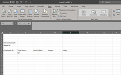
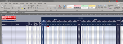
I'm working on two different sheets - the Payroll File 2023 (picture 1), cell B8 will change based on A5 (dropdown list - showing working weeks), taking information from the Construction - Payroll Hrs 2023 (picture 2), starting with cell AK9 (54.00 in TOTAL column). This value will change each time, depending on the week - weeks are displayed in line 5. So if I select week 19 in Payroll File, I should get number 39.5 in total (BM9 - Construction payroll sheet). I am using the below formula but I have a feeling I've set it up for searching the info vertically rather than horizontally.

{IFERROR(INDEX('[Construction Payroll Hrs 2023 - Copy.xlsx]Construction - Payroll Hrs 2023'!$J$9:$AK$9,SMALL(IF('[Construction Payroll Hrs 2023 - Copy.xlsx]Construction - Payroll Hrs 2023'!$J$5:$DR$5=A5,ROW('[Construction Payroll Hrs 2023 - Copy.xlsx]Construction - Payroll Hrs 2023'!$J$9:$AK$9)-MIN(ROW('[Construction Payroll Hrs 2023 - Copy.xlsx]Construction - Payroll Hrs 2023'!$J$9:$AK$9))+1),COLUMNS(A5:A5))),"")}

Any help much appreciated.

Thank you.
Lucie.

 

[awoohaw]

hi, can you help the forum help you? It takes a lot of time for the forum to recreate your data page. Can you please use the xl2bb add (link below) and post a mini worksheet of your data (sanitize it for anonymity please).

 

[Snakehips]

@LucieLiskova I second the above.
However, maybe the below reflects what you are wanting?

Book1.xlsx
	A	B	C	D	E
1
2
3
4	Period Number
5	Week 19
6
7	Employee Id	Total Hours	Hourly Rate	Wages	Salary
8	1	39.5
9	2	99
10	3	23
11	4	0
12	5	0
Sheet3

Cell Formulas
Range	Formula
B8:B12	B8	=IFERROR(INDEX('Construction Payroll Hrs 2023'!J$9:DR$20,MATCH($A8,'Construction Payroll Hrs 2023'!$A$9:$A$20,0),MATCH($A$5,('Construction Payroll Hrs 2023'!J$5:DR$5),0)),"")

Book1.xlsx
	A	B	C	D	E	F	G	H	I	J	K	L	M	N	O	P	Q	R	S	T	U	V	W	X	Y	Z	AA	AB	AC	AD	AE	AF	AG	AH	AI	AJ	AK	AL	AM	AN	AO	AP	AQ	AR	AS	AT	AU	AV	AW	AX	AY	AZ	BA	BB	BC	BD	BE	BF	BG	BH	BI	BJ	BK	BL	BM	BN	BO	BP	BQ	BR	BS	BT	BU	BV	BW	BX	BY	BZ	CA	CB	CC	CD	CE	CF	CG	CH	CI	CJ	CK	CL	CM	CN	CO	CP
1
2
3
4
5																																					Week 18																												Week 19																												Week 20
6
7
8	Emp ID																																				Total																												Total																												Total
9	1																																				54																												39.5																												40
10	2																																				46																												99																												26
11	3																																				37																												23																												40
12	4
13	5
Construction Payroll Hrs 2023

 

[LucieLiskova]

Apologies, see below.

Data from Construction Payroll Hrs 2023 - Copy.xlsx will feed into Payroll File 2023.xlsx. Specifically, Construction Payroll Hrs 2023 - Copy.xlsx the 'TOTAL' column number will change in Payroll File 2023.xlsx based on the dropdown in cell A5 and also needs to check for the employee ID (back in Construction Payroll Hrs 2023 - Copy.xlsx).

So if I select week 18 in Payroll Hrs 2023, it should give me 54.00 for Employee ID 1 'Total Hours' (B7). When selecting week 19, I should see 39.5 in Employee ID 1 'Total Hours'.

@Snakehips thank you for the reply, it didn't work though. I hope the minisheet helps?

Construction Payroll Hrs 2023 - Copy.xlsx
	C	D	E							L	M	N	O	P	Q	R	S	T	U	V	W	X															AM	AN	AO	AP	AQ	AR	AS	AT	AU	AV	AW	AX	AY	AZ															BO
3										PERIOD 10
4
5															Week 18																												Week 19
6										Mon		Tue		Wed		Thu		Fri		Sat		Sun															WEEK 18	Mon		Tue		Wed		Thu		Fri		Sat		Sun															WEEK 19
7										01/05/2023		02/05/2023		03/05/2023		04/05/2023		05/05/2023		06/05/2023		#######																08/05/2023		09/05/2023		10/05/2023		11/05/2023		12/05/2023		13/05/2023		#######
8	Employee ID	First Name	Surname							Shift	O/T	Shift	O/T	Shift	O/T	Shift	O/T	Shift	O/T	First 4 hrs	O/T	O/T															TOTAL	Shift	O/T	Shift	O/T	Shift	O/T	Shift	O/T	Shift	O/T	First 4 hrs	O/T	O/T															TOTAL
9	1									BH	2	SL	1	8	1	8	1	7.5	1	5	2	3															54.00	8		8		8		8		7.5																			39.5
10	2									BH		8		8		8		7.5																			39.50	8		8		8		8		7.5																			39.5
11	3									BH		8		8		8		7.5																			39.50	8		8		8		8		7.5																			39.5
12	4									BH		8		8		8		7.5																			39.50	8		8		8		8		7.5																			39.5
13	5									BH		8		8		8		7.5																			39.50	8		8		8		8		7.5																			39.5
14	6									BH		8		8		8		7.5																			39.50	8		8		8		8		7.5																			39.5
15	7									BH		8		8		8		7.5																			39.50	8		8		8		8		7.5																			39.5
16	8									BH		8		8		8		7.5																			39.50	8		8		8		8		7.5																			39.5
17	9									BH		8		8		8		7.5																			39.50	8		8		8		8		7.5																			39.5
18	10									BH		8		8		8		7.5																			39.50	8		8		8		8		7.5																			39.5
19	11									BH		8		8		8		7.5																			39.50	8		8		8		8		7.5																			39.5
20	12									BH		8		8		8		7.5																			39.50	8		8		8		8		7.5																			39.5
21	13									BH		8		8		8		7.5																			39.50	8		8		8		8		7.5																			39.5
22	14									BH		8		8		8		7.5																			39.50	8		8		8		8		7.5																			39.5
23	15									BH		8		8		8		7.5																			39.50	8		8		8		8		7.5																			39.5
24	16									BH		8		8		8		7.5																			39.50	8		8		8		8		7.5																			39.5
25	17									BH		8		8		8		7.5																			39.50	8		8		8		8		7.5																			39.5
26	18									BH		8		8		8		7.5																			39.50	8		8		8		8		7.5																			39.5
27	19									BH		8		8		8		7.5																			39.50	8		8		8		8		7.5																			39.5
28	20									BH		8		8		8		7.5																			39.50	8		8		8		8		7.5																			39.5
Construction - Payroll Hrs 2023

Cell Formulas
Range	Formula
AM9:AM28,BO9:BO28	AM9	=IF(AH9>=39.5,AH9+AI9+AK9+AC9,(AH9+AC9+AI9+AK9))

Cells with Conditional Formatting
Cell	Condition		Cell Format	Stop If True
AT9:AT28	Cell Value	contains "BH"	text	NO
AT9:AT28	Cell Value	contains "PL"	text	NO
AT9:AT28	Cell Value	contains "SL"	text	NO
AT9:AT28	Cell Value	contains "AL"	text	NO
AR9:AR28	Cell Value	contains "BH"	text	NO
AR9:AR28	Cell Value	contains "PL"	text	NO
AR9:AR28	Cell Value	contains "SL"	text	NO
AR9:AR28	Cell Value	contains "AL"	text	NO
AV9:AV28	Cell Value	contains "BH"	text	NO
AV9:AV28	Cell Value	contains "PL"	text	NO
AV9:AV28	Cell Value	contains "SL"	text	NO
AV9:AV28	Cell Value	contains "AL"	text	NO
AP9:AP28	Cell Value	contains "BH"	text	NO
AP9:AP28	Cell Value	contains "PL"	text	NO
AP9:AP28	Cell Value	contains "SL"	text	NO
AP9:AP28	Cell Value	contains "AL"	text	NO
R9:R28	Cell Value	contains "BH"	text	NO
R9:R28	Cell Value	contains "PL"	text	NO
R9:R28	Cell Value	contains "SL"	text	NO
R9:R28	Cell Value	contains "AL"	text	NO
P9:P28	Cell Value	contains "BH"	text	NO
P9:P28	Cell Value	contains "PL"	text	NO
P9:P28	Cell Value	contains "SL"	text	NO
P9:P28	Cell Value	contains "AL"	text	NO
AZ9:AZ28	Cell Value	contains "BH"	text	NO
AZ9:AZ28	Cell Value	contains "PL"	text	NO
AZ9:AZ28	Cell Value	contains "SL"	text	NO
AZ9:AZ28	Cell Value	contains "AL"	text	NO
AX9:AY28	Cell Value	contains "BH"	text	NO
AX9:AY28	Cell Value	contains "PL"	text	NO
AX9:AY28	Cell Value	contains "SL"	text	NO
AX9:AY28	Cell Value	contains "AL"	text	NO
AN9:AN28	Cell Value	contains "BH"	text	NO
AN9:AN28	Cell Value	contains "PL"	text	NO
AN9:AN28	Cell Value	contains "SL"	text	NO
AN9:AN28	Cell Value	contains "AL"	text	NO
V9:X28	Cell Value	contains "BH"	text	NO
V9:X28	Cell Value	contains "PL"	text	NO
V9:X28	Cell Value	contains "SL"	text	NO
V9:X28	Cell Value	contains "AL"	text	NO
T9:T28	Cell Value	contains "BH"	text	NO
T9:T28	Cell Value	contains "PL"	text	NO
T9:T28	Cell Value	contains "SL"	text	NO
T9:T28	Cell Value	contains "AL"	text	NO
N9:N28	Cell Value	contains "BH"	text	NO
N9:N28	Cell Value	contains "PL"	text	NO
N9:N28	Cell Value	contains "SL"	text	NO
N9:N28	Cell Value	contains "AL"	text	NO
L9:L28	Cell Value	contains "BH"	text	NO
L9:L28	Cell Value	contains "PL"	text	NO
L9:L28	Cell Value	contains "SL"	text	NO
L9:L28	Cell Value	contains "AL"	text	NO

Payroll File 2023..xlsx
	A	B	C	D	E	F	G	H	I	J	K
1
2
3
4	Period Number										Week 18
5	Week 18										Week 19
6											Week 20
7	Employee ID	Total Hours	Hourly Rate	Wages	Salary						Week 21
8	1										Week 22
9	2
10	3
11	4
12	5
13	6
14	7
15	8
16	9
17	10
18	11
19	12
20	13
21	14
22	15
23	16
24	17
25	18
26	19
Payroll File 2023

Cell Formulas
Range	Formula
B8	B8	=IFERROR(INDEX('C:\Users\lucie.liskova\Desktop\[Construction Payroll Hrs 2023 - Copy.xlsx]Construction - Payroll Hrs 2023'!AM$9:DR$20,MATCH($A8,'C:\Users\lucie.liskova\Desktop\[Construction Payroll Hrs 2023 - Copy.xlsx]Construction - Payroll Hrs 2023'!$A$9:$A$20,0),MATCH($A$5,('C:\Users\lucie.liskova\Desktop\[Construction Payroll Hrs 2023 - Copy.xlsx]Construction - Payroll Hrs 2023'!AM$5:DR$5),0)),"")
B9:B26	B9	=IFERROR(INDEX('C:\Users\lucie.liskova\Desktop\[Construction Payroll Hrs 2023 - Copy.xlsx]Construction - Payroll Hrs 2023'!J$9:DR$20,MATCH($A9,'C:\Users\lucie.liskova\Desktop\[Construction Payroll Hrs 2023 - Copy.xlsx]Construction - Payroll Hrs 2023'!$A$9:$A$20,0),MATCH($A$5,('C:\Users\lucie.liskova\Desktop\[Construction Payroll Hrs 2023 - Copy.xlsx]Construction - Payroll Hrs 2023'!J$5:DR$5),0)),"")
Press CTRL+SHIFT+ENTER to enter array formulas.

Cells with Data Validation
Cell	Allow	Criteria
A5	List	=$K$4:$K$8

 

[Alex Blakenburg]

Your XL2BB does not have your data in the same position as your initial picture.

Based on the XL2BB and without creating a second workbook would something like this work for you ?

=INDEX('Construction - Payroll Hrs 2023'!$C$6:$BO$28,
             MATCH($A8,'Construction - Payroll Hrs 2023'!$C$6:$C$28,0),
             MATCH($A$5,'Construction - Payroll Hrs 2023'!$C$6:$BO$6,0))

I have the formula in B8.
And assuming you need to adjust the ranges, the 3 ranges all pivot off the same cell (C6) being the cell that is 2 above Employee ID (same row as the Week 18 which is 2 cells above Total)

If is works just add the IFERROR around it.

 

[LucieLiskova]

Your XL2BB does not have your data in the same position as your initial picture.

Based on the XL2BB and without creating a second workbook would something like this work for you ?

=INDEX('Construction - Payroll Hrs 2023'!$C$6:$BO$28,
             MATCH($A8,'Construction - Payroll Hrs 2023'!$C$6:$C$28,0),
             MATCH($A$5,'Construction - Payroll Hrs 2023'!$C$6:$BO$6,0))

I have the formula in B8.
And assuming you need to adjust the ranges, the 3 ranges all pivot off the same cell (C6) being the cell that is 2 above Employee ID (same row as the Week 18 which is 2 cells above Total)

If is works just add the IFERROR around it.

This is brilliant, Alex. Works just perfect. Thanks so much.

 

[Alex Blakenburg]

You're welcome. Glad we could help.
Having @awoohaw & @Snakehips input helped

 

[LucieLiskova]

Your XL2BB does not have your data in the same position as your initial picture.

Based on the XL2BB and without creating a second workbook would something like this work for you ?

=INDEX('Construction - Payroll Hrs 2023'!$C$6:$BO$28,
             MATCH($A8,'Construction - Payroll Hrs 2023'!$C$6:$C$28,0),
             MATCH($A$5,'Construction - Payroll Hrs 2023'!$C$6:$BO$6,0))

I have the formula in B8.
And assuming you need to adjust the ranges, the 3 ranges all pivot off the same cell (C6) being the cell that is 2 above Employee ID (same row as the Week 18 which is 2 cells above Total)

If is works just add the IFERROR around it.

Hi Alex,

I was trying to apply the same for the rest of the columns in payroll file 2023 - so behind the 'TOTAL' I have few other columns hidden. Behind the employee total hrs I basically want to have a breakdown of overtime, hols, etc. I couldn't make it work and only after a few tries I realized that you based it on the fact that week number is included above the total hours. Is there any other way to make this work for the rest of the columns, you think?

I tried index / match, combination of vlookup / hlookup but nothing works.

I actually posted another thread for it. INDEX / MATCH Used Horizontally & Looking for a Value Based on a Dropdown List

I'd be happy for any help. Thank you very much.


L.