Formula Help (Calendar) Expanded

[Cybrex]

I posted my original question here because it aligned with what was already being discussed (I also was using [B]jtakw[/B] coding as well so it made sense to post there but it was a really old post. So I was told to start my own!)


Hey All, I'm resurrecting this post because I have a question that works off of this (as I'm using this same formula for mine, but for some reason it wouldn't copy correctly across the row so I had to manually update where to target the year for every cell, lol).

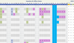
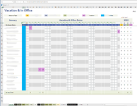
To follow up on this, the calendar we have is used for work. Specifically to track vacation days, what days people are in the office and which office and holidays. I've attached a snippet of what it looks like to help make it easier to understand what I'm looking for.

1) Is there a way to align the day of the month with the correct date. Ie. This screenshot is supposed to be Dec 2024 but for some reason the first day it's showing is a Monday, but when I look at the Calendar it shows the 1st should be a Sunday. So not sure what's happening here?

2) Is there a way to move the column coding we have for the week days/ weekends so they align with the Days of the week at the top instead of me having to copy/paste them to align.

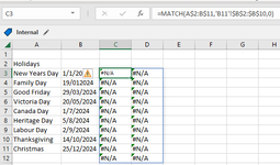
3) The big blue bars shown on here are marked for holidays. Is there a way I can assign another sheet to Canadian holidays and they'll update those blue bars to align with the correct days of those months?

 

[Eric W]

You can pretty much do all that with Conditional Formatting. Put the 1st of the month in cell AH1. The cell is formatted to show just the month and year.

Book1
	A	B	C	D	E	F	G	H	I	J	K	L	M	N	O	P	Q	R	S	T	U	V	W	X	Y	Z	AA	AB	AC	AD	AE	AF	AG	AH
1	Vacation & Office Dates																																	Dec, 2024
2	Sun	Mon	Tue	Wed	Thu	Fri	Sat	Sun	Mon	Tue	Wed	Thu	Fri	Sat	Sun	Mon	Tue	Wed	Thu	Fri	Sat	Sun	Mon	Tue	Wed	Thu	Fri	Sat	Sun	Mon	Tue	O	M	T
3	1	2	3	4	5	6	7	8	9	10	11	12	13	14	15	16	17	18	19	20	21	22	23	24	25	26	27	28	29	30	31
4
5
6
7
8
9
10
11
12
13
14
15
Sheet6

Cell Formulas
Range	Formula
A2:AE2	A2	=SEQUENCE(,DAY(EOMONTH(AH1,0)),AH1)
A3:AE3	A3	=A2#
Dynamic array formulas.

Cells with Conditional Formatting
Cell	Condition		Cell Format	Stop If True
A4:AE15	Expression	=MATCH(A$2,Sheet5!$B$2:$B$10,0)	text	NO
A4:AE15	Expression	=WEEKDAY(A$2,2)>5	text	NO

You have the 2 formulas in A2 and A3. The rest is all cell formatting or Conditional formatting. The holiday list looks like this:

Book1
	A	B
1	Holidays
2	Christmas Eve	12/24/2024
3	Christmas	12/25/2024
4	New Year's Eve	12/31/2024
5
Sheet5

 

[awoohaw]

If you're just concerned with the top two rows, try this:

Book1
	A	B	C	D	E	F	G	H	I	J	K	L	M	N	O	P	Q	R	S	T	U	V	W	X	Y	Z	AA	AB	AC	AD	AE
1	Day 1 of Calendar Month:	2024-12-01
2	Month:	December
3	Year:	2024
4	TRUE
5	Sun	Mon	Tue	Wed	Thu	Fri	Sat	Sun	Mon	Tue	Wed	Thu	Fri	Sat	Sun	Mon	Tue	Wed	Thu	Fri	Sat	Sun	Mon	Tue	Wed	Thu	Fri	Sat	Sun	Mon	Tue
6	1	2	3	4	5	6	7	8	9	10	11	12	13	14	15	16	17	18	19	20	21	22	23	24	25	26	27	28	29	30	31
7
8
9
10
Sheet1

Cell Formulas
Range	Formula
B2	B2	=B1
B3	B3	=B1
A4	A4	=WEEKDAY(A6,2)>5
A5:AE5	A5	=TEXT(DAY(SEQUENCE(1,DAY(EOMONTH(B1,0)),1,1)),"ddd")
A6:AE6	A6	=$B$1+SEQUENCE(1,DAY(EOMONTH(B1,0)),1,1)-1
Dynamic array formulas.

Cells with Conditional Formatting
Cell	Condition		Cell Format	Stop If True
A5:AE10	Expression	=IF(A$6<>"",WEEKDAY(A$6,2)>5)	text	NO

 

[Eric W]

A little more detail. I used the formulas in A2 and A3 so that there would be the right number of days in the month. February would have 28 or 29 days, November 30, etc. The cells A2 to AE2 should have a custom format of ddd and the cells A3 to AE3 should have a custom format of d.

Conditional Formatting allows a cross hatching effect like in your example, but which didn't show up in my mini sheet. You can also select which conditional formatting takes precedence in case a holiday lands on a weekend by changing the order.

 

[Cybrex]

A little more detail. I used the formulas in A2 and A3 so that there would be the right number of days in the month. February would have 28 or 29 days, November 30, etc. The cells A2 to AE2 should have a custom format of ddd and the cells A3 to AE3 should have a custom format of d.

Conditional Formatting allows a cross hatching effect like in your example, but which didn't show up in my mini sheet. You can also select which conditional formatting takes precedence in case a holiday lands on a weekend by changing the order.

Okay, I'm a lot worse at Excel than I thought. lol.
So I was trying on a test sheet based off the original January one (the only one that seems to want to work with the original formula's for some reason).

Breakdown on our calendar tracker
1) 12 sheets for the months each row has an employees name assigned to it with a counter to the right side for when they have marked vacation and what office they were in on what day
2) Summary page that shows the overall count for each employee based on the counters on each month
3) Employee list that is updated when someone joins or leaves the team that than can be updated to each month (has to be done manually)
4) New: Holidays page to hopefully just needs to be updated each year with the new days so the calendar will know what to mark off when the year is changed on each month

I keep getting this Spill notice, and not sure why. I thought it was originally because when I was targeting where I have the year it was a combined amount of cell's and it wasn't understanding what was there so I then just used a single cell in A1 but it still shows Spill. The second formula seems to work fine though it starts off as 0 (which I suspect its due to the #SPILL! error above).

The holiday's section I didn't really understand to where the formula's would go and any time I tried to add it to any page it would continue to try and open a document the moment I pasted it into a cell.

The conditional formatting I think I get what to do. I believe I understand by selecting all the cells, for each day (once the formula's for the days are working properly have it update with, any time it says Mon to Friday change cells to "Colour" When cells show Sat and Sun change cells to cross hatching. So the condition formatting will be based on Row C6 to AG6 ?

Sorry for being a pain, but we had the basic calendar before like in the original post on here and then I went to another team for a year and when I came back someone completely butchered it so I'm trying to make it as simple as possible so when I leave the team again (and I will! lol) there will be no further confusion on how to update it. lol

If it would be easier to upload the excel file to see what I'm doing wrong I can just change out the employees names to a lot of Smiths and remove the name of the offices?

 

[Eric W]

First, let me suggest that you check into the XL2BB tool to post your sample sheet. It makes it easier for the helpers here to work with your data. Yes, you can upload your sample worksheet (cleaned of sensitive information) to a file sharing site and post the link here if you want. But be aware that many people do not like downloading files from the internet for security reasons, so that may limit the people who can help you.

OK, given that, I think I see a few issues based on your picture. First, the SPILL error happens when a spill formula overlaps existing data. Since you left 31 columns open, that should be enough. So there's an issue with the formula. I designed the formula to use the date in the AH1 cell as the starting point. It should be the 1st of the month that you want on this sheet (month, day, year). Then I formatted the cell to just show the month and year. (That's a custom format of "mmm, yyyy".) But on your picture it only shows the year. You have the month on the left. I can adapt the formula, but where is the year saved, and where is the month saved? And what format do they have? Is the year just a number (2024)? Is the month a number (1-12), or the word spelled out ("January")?

Also, there should be NO formulas on the holidays sheet. The other 12 monthly sheets just refer to it with the Conditional Formatting. It kind of looks like you set up the Conditional Formatting for the weekends ok. (Although it doesn't seem to properly match up with the actual weekend dates for 2022. But that could be a result of the SPILL error. We need to get that resolved first.) There's one blue bar, which indicates you have the holiday CF at least partially working too.

Let's get the SPILL error fixed first. Tell me where the month and year are stored on the sheet, and what format they're in.

 

[Cybrex]

First, let me suggest that you check into the XL2BB tool to post your sample sheet. It makes it easier for the helpers here to work with your data. Yes, you can upload your sample worksheet (cleaned of sensitive information) to a file sharing site and post the link here if you want. But be aware that many people do not like downloading files from the internet for security reasons, so that may limit the people who can help you.

OK, given that, I think I see a few issues based on your picture. First, the SPILL error happens when a spill formula overlaps existing data. Since you left 31 columns open, that should be enough. So there's an issue with the formula. I designed the formula to use the date in the AH1 cell as the starting point. It should be the 1st of the month that you want on this sheet (month, day, year). Then I formatted the cell to just show the month and year. (That's a custom format of "mmm, yyyy".) But on your picture it only shows the year. You have the month on the left. I can adapt the formula, but where is the year saved, and where is the month saved? And what format do they have? Is the year just a number (2024)? Is the month a number (1-12), or the word spelled out ("January")?

Also, there should be NO formulas on the holidays sheet. The other 12 monthly sheets just refer to it with the Conditional Formatting. It kind of looks like you set up the Conditional Formatting for the weekends ok. (Although it doesn't seem to properly match up with the actual weekend dates for 2022. But that could be a result of the SPILL error. We need to get that resolved first.) There's one blue bar, which indicates you have the holiday CF at least partially working too.

Let's get the SPILL error fixed first. Tell me where the month and year are stored on the sheet, and what format they're in.

Morning Eric,

That's fair, I won't upload, I don't want people just doing the work, I want to learn and understand it so next time I'll be able to fix it, or even teach someone else how to do it.

So the original design has the month on the Left side of the screen and then we've setup the year on the right. The way it used to work (till someone touched it, lol) was, simply change the year in the top right hand corner and it would know that this is month X (based on the month on the left) and then updated the days/dates accordingly. But its so broken I couldn't get it to work. Even with the January page half working, copying/pasting to the rest of the sheets and correcting the cell's would just fail. So it's pretty much, remove formula's and put in better ones so this doesn't happen again.

Ah! I understand the holidays now, I'll leave that till the last. Conditional Formatting is pretty easy at this point for me now. Once I've got the actual mess fixed that'll be a walk in the park. lol.

 

[Eric W]

OK, if the month (spelled out) is in B4, and the year (year only) is in AH4, then try this:

Book1 (version 1).xlsb
	A	B	C	D	E	F	G	H	I	J	K	L	M	N	O	P	Q	R	S	T	U	V	W	X	Y	Z	AA	AB	AC	AD	AE	AF	AG	AH	AI	AJ
1
2
3			Vacation & Office Dates
4		January	Mon	Tue	Wed	Thu	Fri	Sat	Sun	Mon	Tue	Wed	Thu	Fri	Sat	Sun	Mon	Tue	Wed	Thu	Fri	Sat	Sun	Mon	Tue	Wed	Thu	Fri	Sat	Sun	Mon	Tue	Wed	2024
5			1	2	3	4	5	6	7	8	9	10	11	12	13	14	15	16	17	18	19	20	21	22	23	24	25	26	27	28	29	30	31	O	M	T
6
7
8
9
10
11
12
13
14
15
16
17
18
19
20
21
22
23
Sheet6

Cell Formulas
Range	Formula
C4:AG4	C4	=LET(d,DATEVALUE(B4&" 1, "&AH4),SEQUENCE(,DAY(EOMONTH(d,0)),d))
C5:AG5	C5	=C4#
Dynamic array formulas.

Cells with Conditional Formatting
Cell	Condition		Cell Format	Stop If True
C6:AG23	Expression	=MATCH(C$4,Holidays!$B$3:$B$11,0)	text	YES
C6:AG23	Expression	=(C$4>0)*(WEEKDAY(C$4,2)>5)	text	NO

The custom formatting in C4:AG4 and C5:AG5 is the same as in my previous post. Let us know how this works.

 

[Cybrex]

wtf.xlsx
	A	B	C	D	E	F	G	H	I	J	K	L	M	N	O	P	Q	R	S	T	U	V	W	X	Y	Z	AA	AB	AC	AD	AE	AF	AG	AH	AI	AJ	AK
1		Vacation & In Office
2		Absence Type		O						M						T						V	Vacation						Holiday
3																																		Enter year:
4		January	Vacation & Office Dates																															2022
5			#SPILL!	#VALUE!	###	###	###	###	###	###	###	###	###	###	###	###	###	###	###	###	###	###	###	###	###	###	###	###	###	###	###	###	###
6		Employee Name	0	2	3	4	5	6	7	8	9	10	11	12	13	14	15	16	17	18	19	20	21	22	23	24	25	26	27	28	29	30	31	O	M	T	V
7																																		0	0	0	0
8																																	V	0	0	0	1
Sheet1

Cell Formulas
Range	Formula
C5:AG5	C5	=LET(d,DATEVALUE(B4&" 1, "&AH4),SEQUENCE(,DAY(EOMONTH(d,0)),d))
AH7:AH8	AH7	=COUNTIF('C:\Users\e87111\Desktop\[Vacation & In Office Location 2022.xlsx]Jan'!$C7:$AG7,"O")
AI7:AI8	AI7	=COUNTIF('C:\Users\e87111\Desktop\[Vacation & In Office Location 2022.xlsx]Jan'!$C7:$AG7,"M")
AJ7:AJ8	AJ7	=COUNTIF('C:\Users\e87111\Desktop\[Vacation & In Office Location 2022.xlsx]Jan'!$C7:$AG7,"T")
AK7:AK8	AK7	=COUNTIF('C:\Users\e87111\Desktop\[Vacation & In Office Location 2022.xlsx]Jan'!$C7:$AG7,"V")

Named Ranges
Name	Refers To	Cells
MonthName	=Sheet1!$B$4	C5

Cells with Conditional Formatting
Cell	Condition		Cell Format	Stop If True
C7:AG23	Cell Value	contains "V"	text	NO
AG7:AG23	Expression	=AG7=""	text	YES
AG7:AG23	Expression	=AG7=KeyCustom2	text	YES
AG7:AG23	Expression	=AG7=KeyCustom1	text	YES
AG7:AG23	Expression	=AG7=KeySick	text	YES
AG7:AG23	Expression	=AG7=KeyPersonal	text	YES
AG7:AG23	Expression	=AG7=KeyVacation	text	YES
Z7:Z12	Expression	=Z7=""	text	YES
Z7:Z12	Expression	=Z7=KeyCustom2	text	YES
Z7:Z12	Expression	=Z7=KeyCustom1	text	YES
Z7:Z12	Expression	=Z7=KeySick	text	YES
Z7:Z12	Expression	=Z7=KeyPersonal	text	YES
Z7:Z12	Expression	=Z7=KeyVacation	text	YES
L7:L12	Expression	=L7=""	text	YES
L7:L12	Expression	=L7=KeyCustom2	text	YES
L7:L12	Expression	=L7=KeyCustom1	text	YES
L7:L12	Expression	=L7=KeySick	text	YES
L7:L12	Expression	=L7=KeyPersonal	text	YES
L7:L12	Expression	=L7=KeyVacation	text	YES
S7:S12	Expression	=S7=""	text	YES
S7:S12	Expression	=S7=KeyCustom2	text	YES
S7:S12	Expression	=S7=KeyCustom1	text	YES
S7:S12	Expression	=S7=KeySick	text	YES
S7:S12	Expression	=S7=KeyPersonal	text	YES
S7:S12	Expression	=S7=KeyVacation	text	YES
E7:E14	Expression	=E7=""	text	YES
E7:E14	Expression	=E7=KeyCustom2	text	YES
E7:E14	Expression	=E7=KeyCustom1	text	YES
E7:E14	Expression	=E7=KeySick	text	YES
E7:E14	Expression	=E7=KeyPersonal	text	YES
E7:E14	Expression	=E7=KeyVacation	text	YES
F7:G12	Expression	=F7=""	text	YES
F7:G12	Expression	=F7=KeyCustom2	text	YES
F7:G12	Expression	=F7=KeyCustom1	text	YES
F7:G12	Expression	=F7=KeySick	text	YES
F7:G12	Expression	=F7=KeyPersonal	text	YES
F7:G12	Expression	=F7=KeyVacation	text	YES
M7:N11	Expression	=M7=""	text	YES
M7:N11	Expression	=M7=KeyCustom2	text	YES
M7:N11	Expression	=M7=KeyCustom1	text	YES
M7:N11	Expression	=M7=KeySick	text	YES
M7:N11	Expression	=M7=KeyPersonal	text	YES
M7:N11	Expression	=M7=KeyVacation	text	YES
T7:U11	Expression	=T7=""	text	YES
T7:U11	Expression	=T7=KeyCustom2	text	YES
T7:U11	Expression	=T7=KeyCustom1	text	YES
T7:U11	Expression	=T7=KeySick	text	YES
T7:U11	Expression	=T7=KeyPersonal	text	YES
T7:U11	Expression	=T7=KeyVacation	text	YES
AA7:AB11	Expression	=AA7=""	text	YES
AA7:AB11	Expression	=AA7=KeyCustom2	text	YES
AA7:AB11	Expression	=AA7=KeyCustom1	text	YES
AA7:AB11	Expression	=AA7=KeySick	text	YES
AA7:AB11	Expression	=AA7=KeyPersonal	text	YES
AA7:AB11	Expression	=AA7=KeyVacation	text	YES
H7:I12,K7:K12,R7:R12,Y7:Y12,O7:P17,V7:W17,AC7:AD17	Expression	=H7=""	text	YES
H7:I12,K7:K12,R7:R12,Y7:Y12,O7:P17,V7:W17,AC7:AD17	Expression	=H7=KeyCustom2	text	YES
H7:I12,K7:K12,R7:R12,Y7:Y12,O7:P17,V7:W17,AC7:AD17	Expression	=H7=KeyCustom1	text	YES
H7:I12,K7:K12,R7:R12,Y7:Y12,O7:P17,V7:W17,AC7:AD17	Expression	=H7=KeySick	text	YES
H7:I12,K7:K12,R7:R12,Y7:Y12,O7:P17,V7:W17,AC7:AD17	Expression	=H7=KeyPersonal	text	YES
H7:I12,K7:K12,R7:R12,Y7:Y12,O7:P17,V7:W17,AC7:AD17	Expression	=H7=KeyVacation	text	YES
C7:D10,J7:J17,Q7:Q17,X7:X17,AE7:AF17	Expression	=C7=""	text	YES
C7:D10,J7:J17,Q7:Q17,X7:X17,AE7:AF17	Expression	=C7=KeyCustom2	text	YES
C7:D10,J7:J17,Q7:Q17,X7:X17,AE7:AF17	Expression	=C7=KeyCustom1	text	YES
C7:D10,J7:J17,Q7:Q17,X7:X17,AE7:AF17	Expression	=C7=KeySick	text	YES
C7:D10,J7:J17,Q7:Q17,X7:X17,AE7:AF17	Expression	=C7=KeyPersonal	text	YES
C7:D10,J7:J17,Q7:Q17,X7:X17,AE7:AF17	Expression	=C7=KeyVacation	text	YES

Cells with Data Validation
Cell	Allow	Criteria
B6	Any value

I just installed xl2bb because I'm lost....and I can't even get it to show the calendar....

Exact same issue as before and I even tried to rebuild the calendar from scratch without making any changes to cells and the exact same issues arise. I'm not at a complete loss. lol. I hate not understanding why its not working and not knowing how to fix it.

 

[Eric W]

Based on the minisheet, I found one issue. You're probably familiar with the original philosophy behind formulas. You put a formula in a cell, and it displays a value in that cell. A few years ago Microsoft came up with "Spill" formulas. These formulas can create multiple values, and these values "spill" into adjacent cells. If the adjacent cells already have something in them, you get a SPILL error. And that's what's happening here. I created a Spill formula for the C5 cell, and D5:AG5 already have something in them. So delete everything in D5:AG5, and put this formula

=LET(d,DATEVALUE(B4&" 1, "&AH4),SEQUENCE(,DAY(EOMONTH(d,0)),d))

in C5 ONLY! D5:AG5 will autofill. Do the same with the row below. Clear D6:AG6 and put

=C5#

in C6 ONLY!

Then for the formatting, select C5:AG5, right click on that range, select Format Cells, use the Number tab, click Custom, and in the Type: box put ddd and click OK. Then select C6:AG6, right click on that range, select Format Cells, use the Number tab, click Custom, and in the Type: box put d and click OK.

Let me know how that works. Then we can look at the Conditional Formatting for the weekends and holidays, which both rely on the C5 formula working right.