Formula help INDEX and MATCH Please :)

[BeckyLH88]

Hello all,

I have added a formula, which on the first input returns the right result.

But when I drag this down, it then returns the result of the cell before but the result of the right so therefore moves the look up onto the next month.

Here's my formula:

=SUMIF('[Budget FY2024.xlsx] Budget'!$C$3:$N$3,$E$3,INDEX('[Budget FY2024.xlsx] Budget'!$C$6:$N$133,0,MATCH($B7,'[Budget FY2024.xlsx] Budget'!$B$6:$B$133,0)))

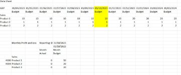
C3 - N3 being the date range
E3 is the date to be looked up
C6 - N133 being the range of data
B7 is the text for example 'staff costs' to look up
B6 - B133 is the text range

So for example:

1st October staff cost is 10, the first field has 10 returned. Formula is then dragged down, the look up changes to office costs, but then it brings the November Staff cost into this figure.


Really appreciate the help. Thank you in advance

 

[steve the fish]

Do you have example data and what you need?

 

[BeckyLH88]

I've mapped out the data type and then below is the result I am seeing from my formula

 

[steve the fish]

Can you copy and paste it so i can paste into excel. Saves me typing...

 

[BeckyLH88]

GBP

01/04/2023​

01/05/2023​

01/06/2023​

01/07/2023​

01/08/2023​

01/09/2023​

01/10/2023​

01/11/2023​

01/12/2023​

01/01/2024​

01/02/2024​

01/03/2024​

Budget

Budget

Budget

Budget

Budget

Budget

Budget

Budget

Budget

Budget

Budget

Budget

Sales

Product 1

10​

10​

10​

10​

10​

10​

10​

20​

20​

20​

20​

20​

Product 2

1​

1​

1​

1​

1​

1​

1​

1​

1​

1​

1​

1​

Product 3

2​

2​

2​

2​

2​

2​

2​

2​

2​

2​

2​

2​

FX Exchange Monthly Profit and loss Reporting Date 31/10/2023 01/10/2023 Translated into GBP Month Month Actual Budget Sales 4000​ Product 1 10 4004​ Product 2 20 Product 3 20

 

[BeckyLH88]

Sorry it's not formatted the way I expected it to when I pasted it in!

 

[steve the fish]

Based on what you have there and copy-pasting it into A1 you could do:

=SUMIF($B$5:$B$7,P17,INDEX($C$5:$N$7,,MATCH(S$13,$C$2:$N$2,0)))

or as you only have one entry per product

=VLOOKUP(P17,$B$5:$N$7,MATCH($S$13,$B$2:$N$2,0))

 

[BeckyLH88]

Sorry unfortunately I do not understand :/

This is my current formula:
=SUMIF('[Budget FY2024.xlsx] Budget'!$C$3:$N$3,$E$3,INDEX('[Budget FY2024.xlsx] Budget'!$C$6:$N$133,0,MATCH($B7,'[Budget FY2024.xlsx] Budget'!$B$6:$B$133,0)))

C3 - N3 being the date range
E3 is the date to be looked up
C6 - N133 being the range of data
B7 is the text for example 'product 1' to look up
B6 - B133 is the text range i.e. product 1, 2 etc

 

[steve the fish]

Im interested in your test data not the formula you have that doesnt work. How does what ive given work on the test data?

 

[BeckyLH88]

It returns an N/A for both, but possibly because I am inputting into A1 but it's not linking to the right cells. I don't particularly understand your formula suggested - sorry!

I am a little rusty, it's been a while since I have used any advanced knowledge!