Formula needed for calculating an average based on other cells.

NamssoB

Board Regular
Joined
Jul 8, 2005
Messages
76
Office Version
  1. 365
  2. 2016
Platform
  1. Windows
Confusing title, I know...here's what I need:

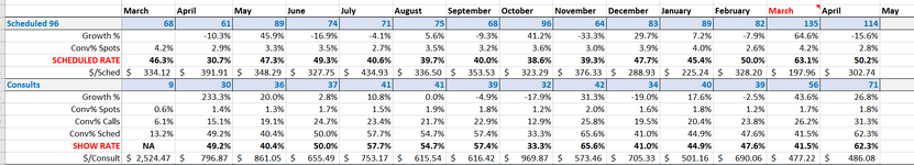
I have a spreadsheet with a label in Column A, and the data is added each month in the columns to the right. For example:

1683648272656.png


What I want:

Cell A22: The label (Scheduled), then appended to this label is the Average of the last 6 values in that row. So A22 *should* say "Scheduled, 94.5 Avg", A27 should say "Consults, 47 Avg".

Using this formula below, I'm getting the wrong average and can't figure out why. What am I doing wrong on this, OR is there a better way to do this?

=CONCATENATE("Scheduled ",AVERAGE(OFFSET($A$22,0,COUNTA($B$22:$Z$22)-6,1,1)))

Also, what happens when I get more than "Z" columns of data? I can change it to ZZ, but that's temporary. is there an absolute way to just find the last column with data?
 

Attachments

  • 1683648233313.png
    1683648233313.png
    47.5 KB · Views: 7

Excel Facts

Back into an answer in Excel
Use Data, What-If Analysis, Goal Seek to find the correct input cell value to reach a desired result
Posting an image is NOT helpful to those trying to provide a solution. Please use XL2BB so that someone trying to help doesn't have to recreate your sheet.
 
Upvote 0
What about A22 being:

Code:
="Scheduled, "&AVERAGE(TAKE(FILTER(B22:AB22,B22:AB22<>""),,-6))&" Avg"

Adjusting the last column to wherever you want to ultimately end.
 
Upvote 0
Another similar option
Excel Formula:
="Scheduled, "&TEXT(AVERAGE(TAKE(FILTER(B22:ZZ22,B22:ZZ22<>""),,-6)),"0.0")&" Avg"
 
Upvote 0
alternatively:
Excel Formula:
="Scheduled, " & AVERAGE(OFFSET(B22,0,COUNT(B22:Z22)-6,1,6))
 
Upvote 0
Set up a named range : =OFFSET(OFFSET(sheet1!$A$1,0,COUNTA(sheet1!$1:$1)-5,1,1),0,0,1,6)

So all you need to do is offset by the number of rows your data is below row 3.

=AVERAGE(OFFSET(namedrange,ROW()-2,0))
 
Upvote 0
a few alternatives to try
="Scheduled "&AVERAGE(TAKE(FILTER(22:22,22:22<>""),,-6))
="Scheduled "&AVERAGE(INDEX(INDEX(B22:Z22,AGGREGATE(14,6,(COLUMN(B22:Z22)-COLUMN(B22)+1)/(B22:Z22<>""),MIN(6,COUNT(B22:Z22)))):Z22,))
="Scheduled "&LET(Last,MATCH(10^35,22:22),AVERAGE(INDEX(22:22,Last):INDEX(22:22,Last-5)))
 
Upvote 0
@Dave Patton won't the 1st & 3rd formulae give a circular reference is they are in A22?
 
Upvote 0
@Dave Patton won't the 1st & 3rd formulae give a circular reference is they are in A22?

Yes probably I would have tested if there was data.
 
Upvote 0
Formulas edited. Please check with your data.
="Scheduled "&ROUND(AVERAGE(INDEX(INDEX(B22:Z22,AGGREGATE(14,6,(COLUMN(B22:Z22)-COLUMN(B22)+1)/(B22:Z22<>""),MIN(6,COUNT(B22:Z22)))):Z22,)),2)

="Scheduled " &ROUND(LET(Last,MATCH(10^35,22:22),AVERAGE(INDEX(22:22,Last):INDEX(22:22,Last-5))),2)

="Scheduled "&ROUND(AVERAGE(TAKE(FILTER(B22:BB22,B22:BB22<>""),,-6)),2)
 
Upvote 0
Solution

Forum statistics

Threads
1,215,387
Messages
6,124,633
Members
449,177
Latest member
Sousanna Aristiadou

We've detected that you are using an adblocker.

We have a great community of people providing Excel help here, but the hosting costs are enormous. You can help keep this site running by allowing ads on MrExcel.com.
Allow Ads at MrExcel

Which adblocker are you using?

Disable AdBlock

Follow these easy steps to disable AdBlock

1)Click on the icon in the browser’s toolbar.
2)Click on the icon in the browser’s toolbar.
2)Click on the "Pause on this site" option.
Go back

Disable AdBlock Plus

Follow these easy steps to disable AdBlock Plus

1)Click on the icon in the browser’s toolbar.
2)Click on the toggle to disable it for "mrexcel.com".
Go back

Disable uBlock Origin

Follow these easy steps to disable uBlock Origin

1)Click on the icon in the browser’s toolbar.
2)Click on the "Power" button.
3)Click on the "Refresh" button.
Go back

Disable uBlock

Follow these easy steps to disable uBlock

1)Click on the icon in the browser’s toolbar.
2)Click on the "Power" button.
3)Click on the "Refresh" button.
Go back
Back
Top