Formula(s) / macro to reduce the digit numbers length of unit measure (UM) part from a string, then to export the new UM section in another column

vladimiratanasiu

Active Member
Joined
Dec 17, 2010
Messages
346
Office Version
  1. 2021
  2. 2019
Platform
  1. Windows
Hello!

I have a very large database, including about 13000 retail products. Each product, depending on the composition and packaging, includes in its string name (column A) data about weight or volume, expressed as UM in litre / kilogram or their smaller unit (miligram / mililitre)- e.g. LIPTON ICE TEA GREEN WHITE PIERSICA 1.5L ; FITNESS CEREALE FRUCTE 225G. The values corresponding to products are expressed by larger (see column A - 1250G, 1800ML etc.) or smaller (idem – 2L, 1KG etc.) values. Giving the integration of database in a SaaS software, the new technical conditions require a standardized system for names of products, with a limited number of characters. It views also the UM elements length, that must be optimized by reducing as much as possible their dimension, and converting the larger length a smaller one. In this sense, it was decided that all values exceeding the thousandth number level (e.g. MIRINDA STRUGURI SI PEPENE GALBEN 1400ML) must be reduced to a smaller word dimension (e.g. MIRINDA STRUGURI SI PEPENE GALBEN 1.4L – column Desired UM results), and other ones, with a large number of digits of UM (e.g. CHIO CHIPS DLGHT SARE 1250G), be converted to a smaller base of UM(CHIO CHIPS DLGHT SARE 1.25KG). The other values from the names of products, not exceeding the hundredth level (e.g. MIRINDA STRUGURI/PEPENE GALBEN 2L, CINI MINIS CEREALE CAPSUNI 500G, PASTA DINTI AQUAFRESH 3-5ANI 50ML etc. ), will keep their initial form. In case of products without UM (e.g. PACHET FUNERAR), they will be transposed in column Desired UM results keeping their original form of column A.

In a second phase, I need to extract separately in cells of column G that part of every converted name from column Desired UM results, showing only quantity and corresponding UM (e.g. 1.6KG, 1.5L etc.). Similarly, the cells of column G, corresponding to products without UM, will be blank. I would be very grateful if you could find a solution (formula, macro), to cover the needs from columns Desired UM results and column G.

Thank you!

Book2.xlsx
ABC
1Column ADesired UM resultsColumn Q
2Basic data content
3METRO CHEF MURATURI ASORTATE 1600GMETRO CHEF MURATURI ASORTATE 1.6KG1.6KG
4MIRINDA STRUGURI SI PEPENE GALBEN 1400MLMIRINDA STRUGURI SI PEPENE GALBEN 1.4L1.4L
5MIRINDA STRUGURI/PEPENE GALBEN 2LMIRINDA STRUGURI/PEPENE GALBEN 2L2L
6LIPTON ICE TEA GREEN WHITE PIERSICA 1.5LLIPTON ICE TEA GREEN WHITE PIERSICA 1.5L1.5L
7CHIO CHIPS DLGHT SARE 1250GCHIO CHIPS DLGHT SARE 1.25KG1.25KG
8FITNESS CEREALE FRUCTE 225GFITNESS CEREALE FRUCTE 225G225G
9SET 12PAHARE 1800MLSET 12PAHARE 1.8L1.8L
10SANOVITA FULGI DE OVAZ 1KGSANOVITA FULGI DE OVAZ 1KG1KG
11PACHET FUNERARPACHET FUNERARBLANK
12CINI MINIS CEREALE CAPSUNI 500GCINI MINIS CEREALE CAPSUNI 500G500G
13PASTA DINTI AQUAFRESH 3-5ANI 50MLPASTA DINTI AQUAFRESH 3-5ANI 50ML50ML
Sheet2
 

Excel Facts

Who is Mr Spreadsheet?
Author John Walkenbach was Mr Spreadsheet until his retirement in June 2019.
Consider Mid with nested InstrRev functions?
mid("METRO CHEF MURATURI ASORTATE 1.6KG",instrrev("METRO CHEF MURATURI ASORTATE 1.6KG"," ")+1) = 1.6KG
You can break that up (simplify?) by assigning the string to a variable, which will probably be a range reference or a variable to which you pass a range reference. It is necessary that your string contains one space before the UM for that to work.
EDIT - just remembered that some strings don't have UM, so back to the coding board...
Does Q actually contain those values or are you just showing them in the post for clarity?
 
Last edited:
Upvote 0
Consider Mid with nested InstrRev functions?
mid("METRO CHEF MURATURI ASORTATE 1.6KG",instrrev("METRO CHEF MURATURI ASORTATE 1.6KG"," ")+1) = 1.6KG
You can break that up (simplify?) by assigning the string to a variable, which will probably be a range reference or a variable to which you pass a range reference. It is necessary that your string contains one space before the UM for that to work.
EDIT - just remembered that some strings don't have UM, so back to the coding board...
Does Q actually contain those values or are you just showing them in the post for clarity?
Thank you for the quick response!

I try to accurately answer your questions / suggestions.

1. I dont't know the InstrRev function(s) and what framework (applicability, complexity, conditions etc.) they suppose. Anyway, I agree if my problem can solved in this way, based on your suggestions / indications of using them.

2. Regarding the variable the string be assigned to, I attach the link Products names.xlsx, where includes the part of database with products. The column I is the source of the original product names, having as a possible range reference a cell of the green ones that I think it could be used as header. As it's seen, it lacks here the column Desired UM results. I inserted it in the previous message in order to clarify the desired results. But it can still be considered, if necessary to, and then I'll copy them back in the original column. Or, if is a macro, it can point the original column, making the necessary changes directly inside it. As for the option of one variable, I can't figure out which could be a proper one. On the other hand, i'lI find very difficult to insert a space before the UM of 13000 products, as long as the letters M (weight / volume) and L(volume)are present within the other words too.

3. I talked with the database administrator, deciding that the strings without UM are rare and could be ignored from formula / macro.

4. Those values posted as example in the Q column are real, but just in limited number. The large data are contained in the linked database. Later edit: The administrator said that modified a little the structure of database. So, the column Q will contain just UM, adding then separately in the column R the corresponding value of each product's volume / weight. I made the necessary changes in the linked document too.

Thank you!
 
Last edited:
Upvote 0
Consider Mid with nested InstrRev functions?
mid("METRO CHEF MURATURI ASORTATE 1.6KG",instrrev("METRO CHEF MURATURI ASORTATE 1.6KG"," ")+1) = 1.6KG
You can break that up (simplify?) by assigning the string to a variable, which will probably be a range reference or a variable to which you pass a range reference. It is necessary that your string contains one space before the UM for that to work.
EDIT - just remembered that some strings don't have UM, so back to the coding board...
Does Q actually contain those values or are you just showing them in the post for clarity?
Hello, Micron!

I found a formula with the MID function, as is shown in the inserted table. It extracts separately the numerical values for the quantity specific to each product. Anyway, when it founds in the content percentages / other words linked with (e.g. 12PAHARE) too, placed before the quantitative ones, it returns only the % / words corresponding value (see the red cells). Do you know to correct this error, and adjust the formula to work properly according with my previous needs?

Thank you!

Book3
AB
1PRODUCTQUANTITY
2CREMA CIOCOLATA LEONA 200G200.00
3CARAFA BISTROT 1L1.00
4ARO CEREALE CACAO BILUTE 250G250.00
5VINETE COAPTE BEL-STO 780G780.00
6BORS BEL-STO 1L1.00
7FITNESS CEREALE FRUCTE 225G225.00
8SET 12PAHARE 180ML12.00
9SANOVITA FULGI DE OVAZ 1KG1.00
10CAMPINA UNT 65% 200G0.65
11CAMPINA FRISCA DIN SMANTANA 35% 1L0.35
12ARO ALCOOL SANITAR 70% 0.5L0.70
13IAURT MERIDIAN 2,8% PET 900G2.00
14SOLE LAPTE CONSUM 3,2% 1L3.00
15DELACO BRANZA PROASPATA 0,2% 250G0.00
Sheet1

 
Last edited:
Upvote 0
I cannot look at your file until later on today at the earliest. However, if you wish to try the following code it might help you. I thought you wanted the UM like 120G and not what you're showing in the red column so that is what I did. Note that since I did not have a sheet to work with, I tested using strings rather than cells but the code contains instructions on how to make it work from a sheet (untested). You would remove the ''' to enable a line. To make the following work in a column, you would follow the instructions to swap the lines and in a sheet cell put =ReturnUMs(A2) and drag that down the column. To use the code as is, in the immediate window you would write
?ReturnUMs("SET 12PAHARE 180ML") and press Enter to test. You should get
180ML as a result.


VBA Code:
'''Function ReturnUMs(rng As Range) As String
Function ReturnUMs(str As String) As String 'disable this line if above is used

Dim strIn As String, strOut As String
Dim intPos As Integer

'''strIn = rng.Value
strIn = str 'disable this line if above is used
intPos = InStrRev(strIn, " ")

strOut = Trim(Mid(strIn, intPos))
If Not Val(strOut) = 0 Then
   ReturnUMs = strOut
Else
   ReturnUMs = strIn
End If

End Function
 
Upvote 0
Hello, Micron!

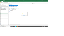
I attached the test file Book4.xlsm . I applied in Sheet 1 the formula =ReturnUMs(A2), returning the results from column E as you said. However, I didn't understand very well the instruction with ?ReturnUMs("SET 12PAHARE 180ML". I inserted the VBA but when try running it generates the error message shown in the the attached photo. Will you have a few minutes to see the attachment and advice me on this problem?

P.S. As you mentioned, the result of the operation should be 180ML. However, I need it gets the value 1,8L, as it's shown in the first table.

Thank you!
 

Attachments

  • Untitled1.png
    Untitled1.png
    113.7 KB · Views: 6
Last edited:
Upvote 0
You have an unnecessary sub line at the top - message means you're missing the end sub, so that's a clue. You don't need it.
I've got construction work going on around the house today, so I have limited time to spend on forums today. Just a few minutes here and there.
 
Upvote 0
You have an unnecessary sub line at the top - message means you're missing the end sub, so that's a clue. You don't need it.
I've got construction work going on around the house today, so I have limited time to spend on forums today. Just a few minutes here and there.
Thank you, Micron, for all your support! The most of results based on the formula and macro are very good.:) However, there are still some issues regarding the final values. In the attached database ( Product names.xlsm ), some products contain UMs inside, not at the end of the string (see the yellow coloured cells). In this case, the final values are returned as the whole string. On the other hand, many products don't include UMs, generating errors or the whole string again in the destination cells . Could you modify the macro, so that the respective cells are empty when such content is exported in them? I noticed gladly that you included the UM buc. (piece/s), too. Similarly, they too meet the same problem if the UM is inside the string.
I wonder and ask you if there is / you know an alternative to extract substrings based on wildcards, that could refine the search and identify as many as possible positions of the UMs inside of the string.
Anyway, thinking you have a lot of experience in VBA and / or Excel, I hope you could help me further on this issue, as your time permits.

Thank you!
 
Last edited:
Upvote 0
I wonder and ask you if there is / you know an alternative to extract substrings based on wildcards, that could refine the search and identify as many as possible positions of the UMs inside of the string.
Possibly VBA RegEx (Regular Expressions), which is something that I gave up trying to learn. I will see what I can do with your issue over the weekend (but it won't involve RegEx).
 
Upvote 0
I don't see an easy code fix. Consider FITNESS CEREALE IAURT 225G GRAU INTEGRAL. If you can easily spot what looks like bad data format, you could edit to
FITNESS CEREALE IAURT GRAU INTEGRAL 225G and run again. At first I considered some sort of method to find numbers coupled with UM's but I see no obvious and relatively simple solution since data like this SET 12PAHARE 180ML contains numbers in the middle but no UM's. I also considered a table of UM's that code could look for but there are numbers coupled with other characters all over the place.

I think you can only take this solution so far - perhaps as far as it is now. IMO, the best solution is one that removes the problem in the first place, and that would be data input at the source.
 
Upvote 0

Forum statistics

Threads
1,215,545
Messages
6,125,450
Members
449,227
Latest member
Gina V

We've detected that you are using an adblocker.

We have a great community of people providing Excel help here, but the hosting costs are enormous. You can help keep this site running by allowing ads on MrExcel.com.
Allow Ads at MrExcel

Which adblocker are you using?

Disable AdBlock

Follow these easy steps to disable AdBlock

1)Click on the icon in the browser’s toolbar.
2)Click on the icon in the browser’s toolbar.
2)Click on the "Pause on this site" option.
Go back

Disable AdBlock Plus

Follow these easy steps to disable AdBlock Plus

1)Click on the icon in the browser’s toolbar.
2)Click on the toggle to disable it for "mrexcel.com".
Go back

Disable uBlock Origin

Follow these easy steps to disable uBlock Origin

1)Click on the icon in the browser’s toolbar.
2)Click on the "Power" button.
3)Click on the "Refresh" button.
Go back

Disable uBlock

Follow these easy steps to disable uBlock

1)Click on the icon in the browser’s toolbar.
2)Click on the "Power" button.
3)Click on the "Refresh" button.
Go back
Back
Top