MrDB4Excel
Active Member
- Joined
- Jan 29, 2004
- Messages
- 334
- Office Version
- 2013
- Platform
- Windows
Is it possible to get, then populate these results to an extra sheet, all values in the rows of columns A:G where the value in column A is Dexc with the use of a formula or function of some type? If this is easier done with VBA then that would be acceptable but I would much rather it work without VBA.
First I need to explain the purpose of this workbook. This is a copy of my June workbook which contains 31 sheets, one for each day.
Every day, in the early morning, I gather all browser history from the previous day by using the executable file (BrowsingHistoryView.exe) I downloaded from View the browsing history of your Web browser
Doing this daily operation enables me to sort and save the browser history I deem important to keep which I do in lieu of other browser history-saving methods. This then allows me to keep my C drive uncluttered with browser history files because I then daily delete all browser history. Thus having a record of what I deem important in an Excel file allows me to easily find some important sites.
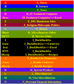
You will see six Xl2bb Mini Sheets as an example of any one of the 31 sheets (month dependent) of which the tabs are named _01, _02, _03… (one for each day of the month)
Now to the point. I would like to have a separate sheet to automatically do what I describe in my first sentence:
“Is it possible to get, then populate these results to an extra sheet, all values in the rows of columns A:G where the value in column A is Dexc with the use of a formula or function of some type?”
Each day may contain many Dexc records or only one or a few and sometimes none.
First I need to explain the purpose of this workbook. This is a copy of my June workbook which contains 31 sheets, one for each day.
Every day, in the early morning, I gather all browser history from the previous day by using the executable file (BrowsingHistoryView.exe) I downloaded from View the browsing history of your Web browser
Doing this daily operation enables me to sort and save the browser history I deem important to keep which I do in lieu of other browser history-saving methods. This then allows me to keep my C drive uncluttered with browser history files because I then daily delete all browser history. Thus having a record of what I deem important in an Excel file allows me to easily find some important sites.
You will see six Xl2bb Mini Sheets as an example of any one of the 31 sheets (month dependent) of which the tabs are named _01, _02, _03… (one for each day of the month)
Now to the point. I would like to have a separate sheet to automatically do what I describe in my first sentence:
“Is it possible to get, then populate these results to an extra sheet, all values in the rows of columns A:G where the value in column A is Dexc with the use of a formula or function of some type?”
Each day may contain many Dexc records or only one or a few and sometimes none.
| 06-JuneTestFile.xlsm | |||||||||
|---|---|---|---|---|---|---|---|---|---|
| A | B | C | D | E | F | G | |||
| 1 | 4 | Visit Time | Site Title-66--136--66 | URL - 77 | Link Category Per Color | Hyperlink | |||
| 2 | Dexc | 6/1/2023 10:13 | Free Online Translator - Preserves your document's layout (PDF, Word, Excel, PowerPoint, OpenOffice, text) | https://www.onlinedoctranslator.com/ | IT-Technical-Computer>>>Excel | https://www.onlinedoctranslator.com/ | |||
| 3 | Dexc | 6/1/2023 05:07 | XLOOKUP two-way exact match - Excel formula | Exceljet | https://exceljet.net/formulas/xlookup-two-way-exact-match | https://exceljet.net/formulas/xlookup-two-way-exact-match | ||||
| 4 | Dexc | 6/1/2023 05:44 | INDEX and MATCH with multiple criteria - Excel formula | Exceljet | https://exceljet.net/formulas/index-and-match-with-multiple-criteria | https://exceljet.net/formulas/index-and-match-with-multiple-criteria | ||||
_01 | |||||||||
| Cell Formulas | ||
|---|---|---|
| Range | Formula | |
| A1 | A1 | =M1 |
| E2 | E2 | =IF((ISERROR(XLOOKUP(A2,'H:\Downloads\Downloads2\RecoverBrowserHistory\ViewBrowserHistory\2023\[05-May.xlsm]01Sort-Types'!$O$1:$O$20,'H:\Downloads\Downloads2\RecoverBrowserHistory\ViewBrowserHistory\2023\[05-May.xlsm]01Sort-Types'!$P$1:$P$20,0))),"",(XLOOKUP(A2,'H:\Downloads\Downloads2\RecoverBrowserHistory\ViewBrowserHistory\2023\[05-May.xlsm]01Sort-Types'!$O$1:$O$20,'H:\Downloads\Downloads2\RecoverBrowserHistory\ViewBrowserHistory\2023\[05-May.xlsm]01Sort-Types'!$P$1:$P$20,0))) |
| E3:E4 | E3 | =IF((ISERROR(XLOOKUP(A3,#REF!$O$1:$O$22,#REF!$P$1:$P$22,0))),"",(XLOOKUP(A3,#REF!$O$1:$O$22,#REF!$P$1:$P$22,0))) |
| G2:G4 | G2 | =HYPERLINK(D2) |
| Cells with Conditional Formatting | ||||
|---|---|---|---|---|
| Cell | Condition | Cell Format | Stop If True | |
| C1 | Cell Value | duplicates | text | NO |
| 06-JuneTestFile.xlsm | |||||||||
|---|---|---|---|---|---|---|---|---|---|
| A | B | C | D | E | F | G | |||
| 1 | 4 | Visit Time | Site Title-66--136--66 | URL - 77 | Link Category Per Color | Hyperlink | |||
| 2 | Dexc | 6/2/2023 05:08 | XLOOKUP and XMATCH: Two New X-Men for Excel < News | SumProduct are experts in Excel Training: Financial Modelling, Strategic Data Modelling, Model Auditing, Planning & Strategy, Training Courses, Tips & Online Knowledgebase | https://www.sumproduct.com/news/article/xlookup-and-xmatch-two-new-x-men-for-excel | https://www.sumproduct.com/news/article/xlookup-and-xmatch-two-new-x-men-for-excel | ||||
| 3 | Dexc | 6/2/2023 05:52 | Excel formula: INDEX and MATCH with multiple criteria - Excelchat | https://www.got-it.ai/solutions/excel-chat/excel-tutorial/lookup/index-and-match-with-multiple-criteria | https://www.got-it.ai/solutions/excel-chat/excel-tutorial/lookup/index-and-match-with-multiple-criteria | ||||
| 4 | Dexc | 6/2/2023 05:09 | XLOOKUP and XMATCH: a new lookup to rule them all (almost) - Excel Quicker | https://www.excelquicker.com/resources/news-sheet/xlookup-and-xmatch-a-new-lookup-to-rule-them-all-almost/ | https://www.excelquicker.com/resources/news-sheet/xlookup-and-xmatch-a-new-lookup-to-rule-them-all-almost/ | ||||
_02 | |||||||||
| Cell Formulas | ||
|---|---|---|
| Range | Formula | |
| A1 | A1 | =M1 |
| E2:E4 | E2 | =IF((ISERROR(XLOOKUP(A2,#REF!$O$1:$O$22,#REF!$P$1:$P$22,0))),"",(XLOOKUP(A2,#REF!$O$1:$O$22,#REF!$P$1:$P$22,0))) |
| G2:G4 | G2 | =HYPERLINK(D2) |
| 06-JuneTestFile.xlsm | |||||||||
|---|---|---|---|---|---|---|---|---|---|
| A | B | C | D | E | F | G | |||
| 1 | 4 | Visit Time | Site Title-66--136--66 | URL - 77 | Link Category Per Color | Hyperlink | |||
| 2 | Dexc | 6/3/2023 07:56 | Enable Automatic Update of Links In Excel - YouTube | https://www.youtube.com/watch?v=G4z6qUrUTjI | https://www.youtube.com/watch?v=G4z6qUrUTjI | ||||
| 3 | Dexc | 6/3/2023 07:53 | Excel Hyperlink Not Working? Here’s How To Fix It | https://www.technewstoday.com/excel-hyperlink-not-working/ | https://www.technewstoday.com/excel-hyperlink-not-working/ | ||||
| 4 | Dexc | 6/3/2023 08:38 | How to Use the IF-THEN Function in Excel | https://www.lifewire.com/entering-data-with-if-function-3123603 | https://www.lifewire.com/entering-data-with-if-function-3123603 | ||||
_03 | |||||||||
| Cell Formulas | ||
|---|---|---|
| Range | Formula | |
| A1 | A1 | =M1 |
| E2:E4 | E2 | =IF((ISERROR(XLOOKUP(A2,#REF!$O$1:$O$22,#REF!$P$1:$P$22,0))),"",(XLOOKUP(A2,#REF!$O$1:$O$22,#REF!$P$1:$P$22,0))) |
| G2:G4 | G2 | =HYPERLINK(D2) |
| 06-JuneTestFile.xlsm | |||||||||
|---|---|---|---|---|---|---|---|---|---|
| A | B | C | D | E | F | G | |||
| 1 | 4 | Visit Time | Site Title-66--136--66 | URL - 77 | Link Category Per Color | Hyperlink | |||
| 2 | Dexc | 6/4/2023 07:55 | Display multiple dates in one cell | MrExcel Message Board | https://www.mrexcel.com/board/threads/display-multiple-dates-in-one-cell.700264/ | https://www.mrexcel.com/board/threads/display-multiple-dates-in-one-cell.700264/ | ||||
| 3 | Dexc | 6/4/2023 08:11 | incorporating a "hard return" within formula | https://www.excelforum.com/excel-formulas-and-functions/624090-incorporating-a-hard-return-within-formula.html | https://www.excelforum.com/excel-formulas-and-functions/624090-incorporating-a-hard-return-within-formula.html | ||||
| 4 | Dexc | 6/4/2023 07:54 | microsoft excel - Multiple dates in the same cell - Super User | https://superuser.com/questions/1579094/multiple-dates-in-the-same-cell | https://superuser.com/questions/1579094/multiple-dates-in-the-same-cell | ||||
_04 | |||||||||
| Cell Formulas | ||
|---|---|---|
| Range | Formula | |
| A1 | A1 | =M1 |
| E2:E4 | E2 | =IF((ISERROR(XLOOKUP(A2,#REF!$O$1:$O$22,#REF!$P$1:$P$22,0))),"",(XLOOKUP(A2,#REF!$O$1:$O$22,#REF!$P$1:$P$22,0))) |
| G2:G4 | G2 | =HYPERLINK(D2) |
| 06-JuneTestFile.xlsm | |||||||||
|---|---|---|---|---|---|---|---|---|---|
| A | B | C | D | E | F | G | |||
| 1 | 4 | Visit Time | Site Title-66--136--66 | URL - 77 | Link Category Per Color | Hyperlink | |||
| 2 | Dexc | 6/5/2023 09:01 | 2 Simple and Easy Ways to Find Duplicates in Excel - wikiHow | https://www.wikihow.com/Find-Duplicates-in-Excel | https://www.wikihow.com/Find-Duplicates-in-Excel | ||||
| 3 | Dexc | 6/5/2023 09:07 | Consolidate duplicates in power query - Microsoft Community Hub | https://techcommunity.microsoft.com/t5/excel/consolidate-duplicates-in-power-query/m-p/2170073 | https://techcommunity.microsoft.com/t5/excel/consolidate-duplicates-in-power-query/m-p/2170073 | ||||
| 4 | Dexc | 6/5/2023 09:02 | excel - Find duplicates from multiple sheets in a workbook - Stack Overflow | https://stackoverflow.com/questions/51810559/find-duplicates-from-multiple-sheets-in-a-workbook | https://stackoverflow.com/questions/51810559/find-duplicates-from-multiple-sheets-in-a-workbook | ||||
_05 | |||||||||
| Cell Formulas | ||
|---|---|---|
| Range | Formula | |
| A1 | A1 | =M1 |
| E2:E4 | E2 | =IF((ISERROR(XLOOKUP(A2,#REF!$O$1:$O$22,#REF!$P$1:$P$22,0))),"",(XLOOKUP(A2,#REF!$O$1:$O$22,#REF!$P$1:$P$22,0))) |
| G2:G4 | G2 | =HYPERLINK(D2) |
| Cells with Conditional Formatting | ||||
|---|---|---|---|---|
| Cell | Condition | Cell Format | Stop If True | |
| C2:D2 | Cell Value | duplicates | text | NO |
| C4:D4 | Cell Value | duplicates | text | NO |
| C3:D3 | Cell Value | duplicates | text | NO |
| C5:D1048576,C1 | Cell Value | duplicates | text | NO |
| 06-JuneTestFile.xlsm | |||||||||
|---|---|---|---|---|---|---|---|---|---|
| A | B | C | D | E | F | G | |||
| 1 | 4 | Visit Time | Site Title-66--136--66 | URL - 77 | Link Category Per Color | Hyperlink | |||
| 2 | Dexc | 6/6/2023 11:55 | Combine Files With Inconsistent Columns In Power Query - YouTube | https://www.youtube.com/watch?v=mg_qLIQjjaM | https://www.youtube.com/watch?v=mg_qLIQjjaM | ||||
| 3 | Dexc | 6/6/2023 12:06 | How To Excel - YouTube | https://www.youtube.com/@HowToExcelBlog | https://www.youtube.com/@HowToExcelBlog | ||||
| 4 | Dexc | 6/6/2023 21:35 | How to Combine Excel Sheets with Power Query - Xelplus - Leila Gharani | https://www.xelplus.com/combine-excel-sheets-power-query/ | https://www.xelplus.com/combine-excel-sheets-power-query/ | ||||
_06 | |||||||||
| Cell Formulas | ||
|---|---|---|
| Range | Formula | |
| A1 | A1 | =M1 |
| E2:E4 | E2 | =IF((ISERROR(XLOOKUP(A2,#REF!$O$1:$O$22,#REF!$P$1:$P$22,0))),"",(XLOOKUP(A2,#REF!$O$1:$O$22,#REF!$P$1:$P$22,0))) |
| G2:G4 | G2 | =HYPERLINK(D2) |