Listing All corresponding dates for a specific value

[FedElecQaEng]

I do not know how to properly explain this but (please note I am unable to post a mini sheet);
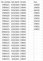
I have a list of several purchase order lines, and date of receipt of the corresponding lines, and the main PO that the lines are a part of. I also have a formula that can get the repeating main PO numbers: Example:

PO LISTING	REC DATE	PO REF		POs
378030/1	4/10/2023	378030		378030
378030/2	4/10/2023	378030		378025
378030/3	4/10/2023	378030		385322
378030/4	4/10/2023	378030		378023
378025/8	5/17/2023	378025		378034
385322/1	8/17/2023	385322		378152
378023/1	6/27/2023	378023		378179
378034/1	3/23/2023	378034		378031
378152/1	6/21/2023	378152		378021
378025/2	3/20/2023	378025		378037
378025/11	7/31/2023	378025		-
378179/1	3/23/2023	378179		-
378031/1	3/22/2023	378031		-
378025/3	4/25/2023	378025		-
378021/2	6/2/2023	378021		-
378031/2	3/22/2023	378031		-
378037/1	4/4/2023	378037		-
378031/3	4/13/2023	378031		-
378037/2	4/4/2023	378037		-
378031/4	4/10/2023	378031		-
378037/3	4/4/2023	378037		-

PO REF Formula:

=IF(A2 = 0,"TBD",LEFT(A2,FIND("/",A2)-1))

POs Formula:

{=IFERROR(INDEX($C$2:$C$22,MATCH(0,COUNTIF($E$1:E1,$C$2:$C$22),0)),"-")}

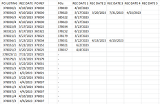
How can I list next to each cell in the POs column all the dates of receipts for each PO? The list of dates can be either all in one cell or spread out among multiple cells, an example being:

Or for example, next to PO 378025 would just be a cell with "5/17/2023, 3/20/2023, 7/31/2023, 4/25/2023"
I would like to do a formula since POs will be added and this is not my entire data.
I would prefer if duplicate dates could be ignored but it will not be an issue if there are duplicate dates listed (PO 378030 would list 4/10/23 four times)
I also do not know how many REC Dates will be for my POs but as long as I can expand the formula I can work with it.

 

[Fluff]

How about

Fluff.xlsm
	A	B	C	D	E	F	G	H	I	J	K
1	PO LISTING	REC DATE	PO REF		POs
2	378030/1	10/04/2023	378030		378030	10/04/2023	10/04/2023	10/04/2023	10/04/2023
3	378030/2	10/04/2023	378030		378025	17/05/2023	20/03/2023	31/07/2023	25/04/2023
4	378030/3	10/04/2023	378030		385322	17/08/2023
5	378030/4	10/04/2023	378030		378023	27/06/2023
6	378025/8	17/05/2023	378025		378034	23/03/2023
7	385322/1	17/08/2023	385322		378152	21/06/2023
8	378023/1	27/06/2023	378023		378179	23/03/2023
9	378034/1	23/03/2023	378034		378031	22/03/2023	22/03/2023	13/04/2023	10/04/2023
10	378152/1	21/06/2023	378152		378021	02/06/2023
11	378025/2	20/03/2023	378025		378037	04/04/2023	04/04/2023	04/04/2023
12	378025/11	31/07/2023	378025
13	378179/1	23/03/2023	378179
14	378031/1	22/03/2023	378031
15	378025/3	25/04/2023	378025
16	378021/2	02/06/2023	378021
17	378031/2	22/03/2023	378031
18	378037/1	04/04/2023	378037
19	378031/3	13/04/2023	378031
20	378037/2	04/04/2023	378037
21	378031/4	10/04/2023	378031
22	378037/3	04/04/2023	378037
23
Sheet5

Cell Formulas
Range	Formula
F2:K11	F2	=IFERROR(INDEX($B:$B,AGGREGATE(15,6,ROW($B$2:$B$100)/($C$2:$C$100=$E2),COLUMNS($F2:F2))),"")

 

[FedElecQaEng]

How about

Fluff.xlsm
	A	B	C	D	E	F	G	H	I	J	K
1	PO LISTING	REC DATE	PO REF		POs
2	378030/1	10/04/2023	378030		378030	10/04/2023	10/04/2023	10/04/2023	10/04/2023
3	378030/2	10/04/2023	378030		378025	17/05/2023	20/03/2023	31/07/2023	25/04/2023
4	378030/3	10/04/2023	378030		385322	17/08/2023
5	378030/4	10/04/2023	378030		378023	27/06/2023
6	378025/8	17/05/2023	378025		378034	23/03/2023
7	385322/1	17/08/2023	385322		378152	21/06/2023
8	378023/1	27/06/2023	378023		378179	23/03/2023
9	378034/1	23/03/2023	378034		378031	22/03/2023	22/03/2023	13/04/2023	10/04/2023
10	378152/1	21/06/2023	378152		378021	02/06/2023
11	378025/2	20/03/2023	378025		378037	04/04/2023	04/04/2023	04/04/2023
12	378025/11	31/07/2023	378025
13	378179/1	23/03/2023	378179
14	378031/1	22/03/2023	378031
15	378025/3	25/04/2023	378025
16	378021/2	02/06/2023	378021
17	378031/2	22/03/2023	378031
18	378037/1	04/04/2023	378037
19	378031/3	13/04/2023	378031
20	378037/2	04/04/2023	378037
21	378031/4	10/04/2023	378031
22	378037/3	04/04/2023	378037
23
Sheet5

Cell Formulas
Range	Formula
F2:K11	F2	=IFERROR(INDEX($B:$B,AGGREGATE(15,6,ROW($B$2:$B$100)/($C$2:$C$100=$E2),COLUMNS($F2:F2))),"")

Thank you Fluff, That worked perfectly.

I never knew about the aggregate function. That function looks to be incredibly useful, I will make note of it and learn how it can be used.

Thank you.

 

[Fluff]

You're welcome & thanks for the feedback.