Go to cell in a column that matches the value of input cell

[rkayz]

Hey EXperta,
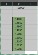
I used this code as below, but I am not getting the desired results, I am getting some columns above and not the exact ones....when I print out the FirstMatchRowNumber, it gives out row#5, whereas it should be 8 from K1, see the image as well

Private Sub Worksheet_Activate()

' Find the last row number in column A.
    Dim lastRow As Long
    With Sheets("T2")
        lastRow = .Cells(.Rows.Count, "K").End(xlUp).Row
    End With

' Find the value you are looking for
    lookupvalue = Worksheets("T2").Range("K1").Value
 
' Select the range you are looking in
    lookuprange = Worksheets("T2").Range("K4:K26" & lastRow)
 
' Find the first matching value, and return the row number
' If there is no matching number, the macro will jump to "ErrorMessageBox"
    On Error GoTo ErrorMesageBox
    FirstMatchRowNumber = WorksheetFunction.Match(lookupvalue, lookuprange, 0)
MsgBox prompt:=FirstMatchRowNumber
' Go to the applicable row.
    Worksheets("T2").Range("K" & FirstMatchRowNumber).Select
Exit Sub



' In case of an unknown number, the macro will show an message box
ErrorMesageBox:
    MsgBox "The number entered in B1 is not known in A1:A" & lastRow
    Exit Sub

End Sub
[/Code}

 

[BSALV]

you have to add an offset = lookuprange.row-1 (here K4, so 4-1 = 3 as you figured out)

Worksheets("T2").Range("K" & FirstMatchRowNumber + lookuprange.row-1 ).Select

 

[rkayz]

Worksheets("T2").Range("K" & FirstMatchRowNumber + lookuprange.row-1 ).Select

Thanks BSalv,
but it goes into the ErrorMesageBox routine as well now? why it should go? and it returns the value of lastRow. it should just select the row matching the value in K1

 

[BSALV]

Worksheets("T2").Range("K" & FirstMatchRowNumber + 3 ).Select

 

[rkayz]

Rich (BB code):
Worksheets("T2").Range("K" & FirstMatchRowNumber [COLOR=rgb(226, 80, 65)][B][SIZE=5]+ 3[/SIZE][/B][/COLOR] ).Select

Thanks Bsalv, that worked.... now further on, I need to hide the other rows above and below, except the selected row + 2 rows above and selected row + 2 rows below

 

[BSALV]

     With Worksheets("T2")
          .Range("K4:K26" & lastrow).EntireRow.Hidden = True     'hide all these rows
          .Range("K" & FirstMatchRowNumber + 3).Offset(-2).Resize(5).EntireRow.Hidden = False     'our row -2 until our row + 2 unhide
     End With

 

[rkayz]

With Worksheets("T2") .Range("K4:K26" & lastrow).EntireRow.Hidden = True 'hide all these rows .Range("K" & FirstMatchRowNumber + 3).Offset(-2).Resize(5).EntireRow.Hidden = False 'our row -2 until our row + 2 unhide End With

Thanks Bsalv, Lemme try it ....

 

[rkayz]

     With Worksheets("T2")
          .Range("K4:K26" & lastrow).EntireRow.Hidden = True     'hide all these rows
          .Range("K" & FirstMatchRowNumber + 3).Offset(-2).Resize(5).EntireRow.Hidden = False     'our row -2 until our row + 2 unhide
     End With

Worked perfectly.... for the current data set.... now in future, If I need to expand the hidden rows above and below (the input selection) to +10 and -10 rows (from the present 2 rows), where do I change? is it the offset value or the resize value?

 

[rkayz]

Worked perfectly.... for the current data set.... now in future, If I need to expand the hidden rows above and below (the input selection) to +10 and -10 rows (from the present 2 rows), where do I change? is it the offset value or the resize value?

Got this nailed, tried few times and was able to fix it.... Thanks Again Bsalv...
Finally, If I need to assign this to a button "Analyze" how do I do it??

 

[rkayz]

Got this nailed, tried few times and was able to fix it.... Thanks Again Bsalv...
Finally, If I need to assign this to a button "Analyze" how do I do it??

even got this fixed.... did a little playing around......phew...!!
now a practical problem.....my actual production sheet (not the testing one on which I built this code), has multiple values found as a result of the input cell "K2", but I need just the first one, or better skip all of the same values as K2, and then hide the rest above and below the found value