Google Sheets Conditional Format with Formula

debapple

New Member
Joined
Dec 1, 2021
Messages
2
Office Version
  1. 365
Platform
  1. MacOS
Hello everyone,

I have a Google Sheet that I need to apply a conditional format to using a formula.

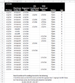
If Cell D3 and E3 are blank and cell G3 is greater than 7, then I need cell B3 to highlight yellow. I have attached a screen shot of an example. Any help is much appreciated!
 

Attachments

  • Screen Shot 2022-01-11 at 10.30.51 AM.png
    Screen Shot 2022-01-11 at 10.30.51 AM.png
    140.5 KB · Views: 15

Excel Facts

Get help while writing formula
Click the italics "fx" icon to the left of the formula bar to open the Functions Arguments dialog. Help is displayed for each argument.
Select b3 downwards & try this formula
Excel Formula:
=AND(D3="",E3="",G3>7)
 
Upvote 0

Forum statistics

Threads
1,215,842
Messages
6,127,227
Members
449,371
Latest member
strawberrish

We've detected that you are using an adblocker.

We have a great community of people providing Excel help here, but the hosting costs are enormous. You can help keep this site running by allowing ads on MrExcel.com.
Allow Ads at MrExcel

Which adblocker are you using?

Disable AdBlock

Follow these easy steps to disable AdBlock

1)Click on the icon in the browser’s toolbar.
2)Click on the icon in the browser’s toolbar.
2)Click on the "Pause on this site" option.
Go back

Disable AdBlock Plus

Follow these easy steps to disable AdBlock Plus

1)Click on the icon in the browser’s toolbar.
2)Click on the toggle to disable it for "mrexcel.com".
Go back

Disable uBlock Origin

Follow these easy steps to disable uBlock Origin

1)Click on the icon in the browser’s toolbar.
2)Click on the "Power" button.
3)Click on the "Refresh" button.
Go back

Disable uBlock

Follow these easy steps to disable uBlock

1)Click on the icon in the browser’s toolbar.
2)Click on the "Power" button.
3)Click on the "Refresh" button.
Go back
Back
Top