Group data from column into separate rows horizontally

[chhantelravi]

Hi Everyone,

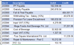
I have a data file which looks like below attachment.

I need to modify it as per my report format which is attached below.

Its really time consuming and hectic for huge files. So can anyone have any idea how to do this?
I would really appreciate help from excel geniuses..
Thanks
Ravi

 

[chhantelravi]

Just looked at this again and not sure why I made it like that. The formula for columns H, I, J, .. could be simpler ..

chhantelravi 2020-08-12 1.xlsm
	A	B	C	D	E	F	G	H	I	J
1		Original format				Required Format
2	Vr ref	Account Name	Dr. Amount	Cr. Amount		Account Name		transaction1	transaction2	transaction3
3	1	Labour Charges	266111.1111			Labour Charges	1	266111.11
4	1	Labour Charges Payable		263450		Labour Charges Payable	1	(263450.00)
5	1	Withholding Tax - SST (1%)		2661.111111		Withholding Tax - SST (1%)	1	(2661.11)
6	2	Intercompany Transactions - SMSK- TIGER	60000			Intercompany Transactions - SMSK- TIGER	2		60000.00
7	2	TDS Receivables	1500			TDS Receivables	2		1500.00
8	2	Sundry Debtros Control Account		61500		Sundry Debtros Control Account	2		(61500.00)
9	3	Intercompany Transactions	190000			Intercompany Transactions	3			190000.00
10	3	TDS Receivables	30000			TDS Receivables	3			30000.00
11	3	Sundry Debtros Control Account		220000		Sundry Debtros Control Account	3			(220000.00)
Sheet3

Cell Formulas
Range	Formula
F3:F11	F3	=B3
G3:G11	G3	=G2+(A3<>A2)
H3:J11	H3	=IF(COLUMNS($H:H)=$G3,IF($D3="",$C3,-$D3),"")

.. or if columns C:D are not formulas ..

chhantelravi 2020-08-12 1.xlsm
	A	B	C	D	E	F	G	H	I	J
2	Vr ref	Account Name	Dr. Amount	Cr. Amount		Account Name		transaction1	transaction2	transaction3
3	1	Labour Charges	266111.1111			Labour Charges	1	266111.11
4	1	Labour Charges Payable		263450		Labour Charges Payable	1	(263450.00)
5	1	Withholding Tax - SST (1%)		2661.111111		Withholding Tax - SST (1%)	1	(2661.11)
6	2	Intercompany Transactions - SMSK- TIGER	60000			Intercompany Transactions - SMSK- TIGER	2		60000.00
7	2	TDS Receivables	1500			TDS Receivables	2		1500.00
8	2	Sundry Debtros Control Account		61500		Sundry Debtros Control Account	2		(61500.00)
9	3	Intercompany Transactions	190000			Intercompany Transactions	3			190000.00
10	3	TDS Receivables	30000			TDS Receivables	3			30000.00
11	3	Sundry Debtros Control Account		220000		Sundry Debtros Control Account	3			(220000.00)
Sheet4

Cell Formulas
Range	Formula
F3:F11	F3	=B3
G3:G11	G3	=G2+(A3<>A2)
H3:J11	H3	=IF(COLUMNS($H:H)=$G3,$C3-$D3,"")

Thanks again Peter. I have already did it to make it simple.
But as I was working on it, I was stuck with another problem. Thanks to you I used your logic and make it work.
You used Vr. ref column to drive the formula, mean with column function, you counted numbers and if its equal to Vr. ref column value it would give "+" or "-" figures. For example, the function will work only if "=column(H:H)=G3", it would return value or else 0.
But if I am working for any month, Say December, then Voucher ref will start from 1. So I have to perform it in 3 steps to get required format.
First I have to summarise total voucher number and give them serial number from 1. Then with vlookup, take serial number reference and finally use your formula.
I have attached a sample for your ref.

Excel working.xlsx
	A	B	C	D	E	F	G	H	I	J	K	L	M	N	O
1		Original format								Report format
2	Vr ref	Account Name	Dr. Amount	Cr. Amount		Vr ref	S.No.		Vr ref	Account Name		Transaction1	Transaction2	Transaction3	Transaction4
3	JV2048	Labour Charges	266,111.11			JV2048	1		JV2048	Labour Charges	1	266111.1111
4	JV2048	Labour Charges Payable		263,450.00		JV2049	2		JV2048	Labour Charges Payable	1	-263450
5	JV2048	Withholding Tax - SST (1%)		2,661.11		JV2050	3		JV2048	Withholding Tax - SST (1%)	1	-2661.111111
6	JV2049	Intercompany Transactions - SMSK- TIGER	60,000.00			JV2051	4		JV2049	Intercompany Transactions - SMSK- TIGER	2		60000
7	JV2049	TDS Receivables	1,500.00						JV2049	TDS Receivables	2		1500
8	JV2049	Sundry Debtros Control Account		61,500.00					JV2049	Sundry Debtros Control Account	2		-61500
9	JV2050	Intercompany Transactions	190,000.00						JV2050	Intercompany Transactions	3			190000
10	JV2050	TDS Receivables	30,000.00						JV2050	TDS Receivables	3			30000
11	JV2050	Sundry Debtros Control Account		220,000.00					JV2050	Sundry Debtros Control Account	3			-220000
12	JV2050	Employee Salary	100,000.00						JV2050	Employee Salary	3			100000
13	JV2050	PF - Employers Contribution	10,000.00						JV2050	PF - Employers Contribution	3			10000
14	JV2050	Gratuity	10,000.00						JV2050	Gratuity	3			10000
15	JV2050	Accomodation Allowance	50,000.00						JV2050	Accomodation Allowance	3			50000
16	JV2050	Salary Payable		115,000.00					JV2050	Salary Payable	3			-115000
17	JV2050	Withholding Tax - SST (1%)		10,000.00					JV2050	Withholding Tax - SST (1%)	3			-10000
18	JV2050	Withholding Tax - Salary (15%)		25,000.00					JV2050	Withholding Tax - Salary (15%)	3			-25000
19	JV2050	PF Payable		10,000.00					JV2050	PF Payable	3			-10000
20	JV2050	Gratuity Payable		10,000.00					JV2050	Gratuity Payable	3			-10000
21	JV2051	NSBL-CA-BHW	60,000.00						JV2051	NSBL-CA-BHW	4				60000
22	JV2051	PCBL - BHW_Account		60,000.00					JV2051	PCBL - BHW_Account	4				-60000
Sheet4

Cell Formulas
Range	Formula
K3:K22	K3	=VLOOKUP(I3,$F$3:$G$6,2,0)
L3:O22	L3	=IF(COLUMNS($L:L)=$K3,IF($D3="",$C3,-$D3),"")

I am trying to do this without Vr. ref.
From your previous question "what trigger this?", There is nothing to trigger. Management want transaction report in this format. So I am working on it.
Thanks

 

[Peter_SSs]

But if I am working for any month, Say December, then Voucher ref will start from 1. So I have to perform it in 3 steps to get required format.
First I have to summarise total voucher number and give them serial number from 1.

Why do you have to do that? If you use my formulas as they were it works doesn't it?

Here is your sheet from post 11. I have removed that lookup data from columns F:G and replaced your column K VLOOKUP with the simple formula I posted before (this time I have pointed it at column I but column A would still work too.). Results look the same to me.

chhantelravi 2020-08-12 1.xlsm
	A	B	C	D	E	F	G	H	I	J	K	L	M	N	O
1		Original format								Report format
2	Vr ref	Account Name	Dr. Amount	Cr. Amount					Vr ref	Account Name		Transaction1	Transaction2	Transaction3	Transaction4
3	JV2048	Labour Charges	266111.1111						JV2048	Labour Charges	1	266111.1111
4	JV2048	Labour Charges Payable		263450					JV2048	Labour Charges Payable	1	-263450
5	JV2048	Withholding Tax - SST (1%)		2661.111111					JV2048	Withholding Tax - SST (1%)	1	-2661.111111
6	JV2049	Intercompany Transactions - SMSK- TIGER	60000						JV2049	Intercompany Transactions - SMSK- TIGER	2		60000
7	JV2049	TDS Receivables	1500						JV2049	TDS Receivables	2		1500
8	JV2049	Sundry Debtros Control Account		61500					JV2049	Sundry Debtros Control Account	2		-61500
9	JV2050	Intercompany Transactions	190000						JV2050	Intercompany Transactions	3			190000
10	JV2050	TDS Receivables	30000						JV2050	TDS Receivables	3			30000
11	JV2050	Sundry Debtros Control Account		220000					JV2050	Sundry Debtros Control Account	3			-220000
12	JV2050	Employee Salary	100000						JV2050	Employee Salary	3			100000
13	JV2050	PF - Employers Contribution	10000						JV2050	PF - Employers Contribution	3			10000
14	JV2050	Gratuity	10000						JV2050	Gratuity	3			10000
15	JV2050	Accomodation Allowance	50000						JV2050	Accomodation Allowance	3			50000
16	JV2050	Salary Payable		115000					JV2050	Salary Payable	3			-115000
17	JV2050	Withholding Tax - SST (1%)		10000					JV2050	Withholding Tax - SST (1%)	3			-10000
18	JV2050	Withholding Tax - Salary (15%)		25000					JV2050	Withholding Tax - Salary (15%)	3			-25000
19	JV2050	PF Payable		10000					JV2050	PF Payable	3			-10000
20	JV2050	Gratuity Payable		10000					JV2050	Gratuity Payable	3			-10000
21	JV2051	NSBL-CA-BHW	60000						JV2051	NSBL-CA-BHW	4				60000
22	JV2051	PCBL - BHW_Account		60000					JV2051	PCBL - BHW_Account	4				-60000
Sheet5 (2)

Cell Formulas
Range	Formula
K3:K22	K3	=K2+(I3<>I2)
L3:O22	L3	=IF(COLUMNS($L:L)=$K3,IF($D3="",$C3,-$D3),"")