Help with a large spreadsheet - converting to columns based on cell value

[retroisbest]

Hi there,
I currently have a large spreadsheet with approx 22,000 rows, 1 column.

What i would like to do is split this one column so it reflects the fieldnames in this single column

The format of the fields :

name: cell value
a: cell value
b: cell value
c: cell value
d: cell value
name: cell value
a:cell value
b:cell value
c:cell value
d:cell value
a:cell value
b:cell value
c:cell value
d:cell value
name: cell value
a:cell value
b:cell value
c:cell value
d:cell value
a:cell value
b:cell value
c:cell value
(Some of the a: - d: fields are repeated in series up to 20 times before we get to a new name: field)
Trying to split on delimiter does not work, I can transpose this one column into one row but again I cant work out how to split the row based off name: field

If i can split the one column into name: | a: | b:| c: | d: columns then i can import this data into an SQL table.


Thankyou for the help and hope the above makes sense.
d:cell value
a:cell value
b:cell value
c:cell value
d:cell value

 

[retroisbest]

Heres some test data (please note field names and data has been changed for posting purposes)

test data.xlsx
	A
1	name: jsmith@test.com
2	a: test (1/5)
3	b: 2021-04-27T02:57:27.156Z
4	c: 330993702388
5	d: COMPLETE
6	e: 106294578281276416052
7	a: test (2/5)
8	b: 2020-12-27T02:55:33.723Z
9	c: 220365365121
10	d:COMPLETE
11	e: 106294578281276416052
12	name: bsmith@test.com
13	a:jcbclb@hotmail.com (1/3)
14	b: 2021-04-27T02:59:04.906Z
15	c:330994437347
16	d:COMPLETE
17	e: 100596666091754468400
18	a: test (2/3)
19	b: 2020-12-27T02:57:06.421Z
20	c: 220365508293
21	d: COMPLETE
22	e: 100596666091754468400
23	a: test (3/3)
24	b: 2020-08-28T09:23:20.289Z
25	c: 152355899161
26	d: COMPLETE
27	e: 100596666091754468400
Sheet1

 

[retroisbest]

I have managed to do this by using "Power Query Editor"

Step 1
First create a custom column with if statement
if Text.Contains([Column1], "Name:") then 1 else 0
New column created with a 1 next to each field of Name:

Step 2
added index column (from 1)

Step 3
Created a custom column which is a list, this list is going to associated all the rows which belong to the record eg the first 12 rows all belong to PersonA
List.Sum(List.FirstN(#"Added Index"[Custom],[Index]))
(we reference a step here so make sure #"Added Index" exists as a step)

Step 4
Filter first column (hide empty)

Step 5
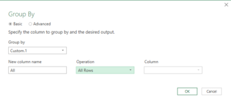
Added "Group By"
(Group by "custom.1" > operation "All Rows")

Step 6
Add an index column to all recently grouped tables

Table.AddIndexColumn([All],"ColIden",1)
This adds an index column called ColIden starting at number 1 and inserts it in every table

Step 7
expand the new table column and select two columns, the newly added coliden column and column1 (this is our original stacked column full of data) removed custom label

Step 8
Delete column "All"

Step 9
Create pivot column select ColIden column then transform > pivot column
Change column value to main data column (which is column1)
Click advanced options select do not aggregate