Help with Excel Text to Column

Maverick27

Active Member
Joined
Sep 23, 2010
Messages
329
Office Version
  1. 2013
Platform
  1. Windows
G'Day Excel Gurus

I need help in converting selective cell data from Text to Column.

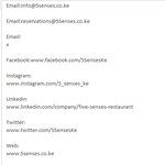
The Column AF data looks the screenshot below:

excel-data.jpg


Anyone care to share a Macro Code (or Excel Function) to convert Text to Column for the following data :
  • Email ( 1st instance )
  • Facebook
  • Instagram
  • Web
The Final excel output should look like:

excel-data-final.jpg


Thanks in Advance.
 

Attachments

  • excel-data.jpg
    excel-data.jpg
    27.5 KB · Views: 11
Using your original columns, it would be as below. Note: I had forgotten that I had to amend the formula to use contains rather than starts-with due to the spaces after the semicolons:

Book2
AFAGAHAIAJ
1EmailFacebookInstagramWeb
2Email:info@5senses.co.ke ; Email:reservations@5Senses.co.ke ; Email:x ; Facebook:www.facebook.com/5SensesKe ; Instagram:www.instagram.com/5_senses_ke ; Linkedin:www.linkedin.com/company/five-senses-restaurant ; Twitter: www.twitter.com/5SensesKe ; Web: www.5senses.co.keinfo@5senses.co.kewww.facebook.com/5SensesKewww.instagram.com/5_senses_kewww.5senses.co.ke
Sheet1
 
Upvote 0

Excel Facts

What does custom number format of ;;; mean?
Three semi-colons will hide the value in the cell. Although most people use white font instead.
Using your original columns, it would be as below. Note: I had forgotten that I had to amend the formula to use contains rather than starts-with due to the spaces after the semicolons:

Book2
AFAGAHAIAJ
1EmailFacebookInstagramWeb
2Email:info@5senses.co.ke ; Email:reservations@5Senses.co.ke ; Email:x ; Facebook:www.facebook.com/5SensesKe ; Instagram:www.instagram.com/5_senses_ke ; Linkedin:www.linkedin.com/company/five-senses-restaurant ; Twitter: www.twitter.com/5SensesKe ; Web: www.5senses.co.keinfo@5senses.co.kewww.facebook.com/5SensesKewww.instagram.com/5_senses_kewww.5senses.co.ke
Sheet1
Great Stuff !!

I'll try it from my end.
 
Upvote 0
You seem to be quite a long way down the formula path but in case it doesn't end up working for you.
Here is a VBA option.

VBA Code:
Sub SplitData()

    Dim shtData As Worksheet
    Dim arrSplitCat As Variant
    Dim arrSplitDetail
    Dim lr As Long, i As Long, j  As Long
    Dim rngData As Range, arrData As Variant, rngOut As Range, arrOut As Variant
    Dim iEmail As Long
    
    Set shtData = ActiveSheet
    With shtData
        lr = .Range("AF" & Rows.Count).End(xlUp).Row
        Set rngData = .Range(.Cells(2, "AF"), .Cells(lr, "AF"))
        arrData = rngData
        Set rngOut = .Cells(2, "AG")
    End With
    
    ReDim arrOut(1 To UBound(arrData), 1 To 5)
    
    For i = 1 To UBound(arrData)
        iEmail = 1
        arrSplitCat = Split(arrData(i, 1), ";")
        For j = 0 To UBound(arrSplitCat)
            arrSplitDetail = Split(arrSplitCat(j), ":")
            Select Case Trim(arrSplitDetail(0))
            
                Case "Email"
                    If iEmail < 3 Then
                        arrOut(i, iEmail) = Trim(arrSplitDetail(1))
                        iEmail = iEmail + 1
                    End If
                Case "Facebook"
                    arrOut(i, 3) = Trim(arrSplitDetail(1))
                Case "Instagram"
                    arrOut(i, 4) = Trim(arrSplitDetail(1))
                Case "Web"
                    arrOut(i, 5) = Trim(arrSplitDetail(1))
                Case Else
                    ' do nothing
            End Select
        Next j
    Next i
    
    Set rngOut = rngOut.Resize(UBound(arrOut, 1), UBound(arrOut, 2))
    With rngOut
        .FormulaR1C1 = arrOut
        .Columns.AutoFit
    End With

    Dim rCell As Range
        For Each rCell In rngOut.Resize(, 2)
        shtData.Hyperlinks.Add anchor:=rCell, Address:="mailto:" & rCell.Value
    Next rCell
    
    For Each rCell In rngOut.Offset(, 2).Resize(rngOut.Rows.Count, rngOut.Columns.Count - 2)
        shtData.Hyperlinks.Add anchor:=rCell, Address:="http://" & rCell.Value
    Next rCell

End Sub
 
Upvote 0
Using your original columns, it would be as below. Note: I had forgotten that I had to amend the formula to use contains rather than starts-with due to the spaces after the semicolons:

Book2
AFAGAHAIAJ
1EmailFacebookInstagramWeb
2Email:info@5senses.co.ke ; Email:reservations@5Senses.co.ke ; Email:x ; Facebook:www.facebook.com/5SensesKe ; Instagram:www.instagram.com/5_senses_ke ; Linkedin:www.linkedin.com/company/five-senses-restaurant ; Twitter: www.twitter.com/5SensesKe ; Web: www.5senses.co.keinfo@5senses.co.kewww.facebook.com/5SensesKewww.instagram.com/5_senses_kewww.5senses.co.ke
Sheet1
Hi Rory - the Function works for some cells since that data is not consistent.

Thanks all the same.
 
Upvote 0
You seem to be quite a long way down the formula path but in case it doesn't end up working for you.
Here is a VBA option.

VBA Code:
Sub SplitData()

    Dim shtData As Worksheet
    Dim arrSplitCat As Variant
    Dim arrSplitDetail
    Dim lr As Long, i As Long, j  As Long
    Dim rngData As Range, arrData As Variant, rngOut As Range, arrOut As Variant
    Dim iEmail As Long
   
    Set shtData = ActiveSheet
    With shtData
        lr = .Range("AF" & Rows.Count).End(xlUp).Row
        Set rngData = .Range(.Cells(2, "AF"), .Cells(lr, "AF"))
        arrData = rngData
        Set rngOut = .Cells(2, "AG")
    End With
   
    ReDim arrOut(1 To UBound(arrData), 1 To 5)
   
    For i = 1 To UBound(arrData)
        iEmail = 1
        arrSplitCat = Split(arrData(i, 1), ";")
        For j = 0 To UBound(arrSplitCat)
            arrSplitDetail = Split(arrSplitCat(j), ":")
            Select Case Trim(arrSplitDetail(0))
           
                Case "Email"
                    If iEmail < 3 Then
                        arrOut(i, iEmail) = Trim(arrSplitDetail(1))
                        iEmail = iEmail + 1
                    End If
                Case "Facebook"
                    arrOut(i, 3) = Trim(arrSplitDetail(1))
                Case "Instagram"
                    arrOut(i, 4) = Trim(arrSplitDetail(1))
                Case "Web"
                    arrOut(i, 5) = Trim(arrSplitDetail(1))
                Case Else
                    ' do nothing
            End Select
        Next j
    Next i
   
    Set rngOut = rngOut.Resize(UBound(arrOut, 1), UBound(arrOut, 2))
    With rngOut
        .FormulaR1C1 = arrOut
        .Columns.AutoFit
    End With

    Dim rCell As Range
        For Each rCell In rngOut.Resize(, 2)
        shtData.Hyperlinks.Add anchor:=rCell, Address:="mailto:" & rCell.Value
    Next rCell
   
    For Each rCell In rngOut.Offset(, 2).Resize(rngOut.Rows.Count, rngOut.Columns.Count - 2)
        shtData.Hyperlinks.Add anchor:=rCell, Address:="http://" & rCell.Value
    Next rCell

End Sub

Hi Alex - The Code works like a charm !! Great Stuff !!

Can you pls edit the code to incorporate the data string for Twitter ?

Thanks in Advance.
 
Upvote 0
You mean some are comma separated rather than semicolon?
 
Upvote 0
I'm surprised the code doesn't have an issue then since it also splits on semicolons. Can't you just do a Find/Replace on the column first to swap commas for semicolons?
 
Upvote 0

Forum statistics

Threads
1,215,038
Messages
6,122,798
Members
449,095
Latest member
m_smith_solihull

We've detected that you are using an adblocker.

We have a great community of people providing Excel help here, but the hosting costs are enormous. You can help keep this site running by allowing ads on MrExcel.com.
Allow Ads at MrExcel

Which adblocker are you using?

Disable AdBlock

Follow these easy steps to disable AdBlock

1)Click on the icon in the browser’s toolbar.
2)Click on the icon in the browser’s toolbar.
2)Click on the "Pause on this site" option.
Go back

Disable AdBlock Plus

Follow these easy steps to disable AdBlock Plus

1)Click on the icon in the browser’s toolbar.
2)Click on the toggle to disable it for "mrexcel.com".
Go back

Disable uBlock Origin

Follow these easy steps to disable uBlock Origin

1)Click on the icon in the browser’s toolbar.
2)Click on the "Power" button.
3)Click on the "Refresh" button.
Go back

Disable uBlock

Follow these easy steps to disable uBlock

1)Click on the icon in the browser’s toolbar.
2)Click on the "Power" button.
3)Click on the "Refresh" button.
Go back
Back
Top