Help With Formula

MickB

New Member
Joined
Oct 21, 2020
Messages
6
Office Version
  1. 2007
Platform
  1. Windows
Hi,

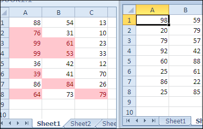
On Sheet 1 under Column B, I have a list part numbers that are defective.
On Sheets 2, 3, 4, 5 etc...... under Column O, I have blank cells to enter part numbers - if a number is entered into any cell under Column O that matches any of the defective part numbers in Sheet 1 Column B I would like the adjacent cell in Column P to fill red (as a warning flag).

What formula would work?

Thanks Mick
 

Excel Facts

Format cells as date
Select range and press Ctrl+Shift+3 to format cells as date. (Shift 3 is the # sign which sort of looks like a small calendar).

Forum statistics

Threads
1,214,991
Messages
6,122,628
Members
449,095
Latest member
bsb1122

We've detected that you are using an adblocker.

We have a great community of people providing Excel help here, but the hosting costs are enormous. You can help keep this site running by allowing ads on MrExcel.com.
Allow Ads at MrExcel

Which adblocker are you using?

Disable AdBlock

Follow these easy steps to disable AdBlock

1)Click on the icon in the browser’s toolbar.
2)Click on the icon in the browser’s toolbar.
2)Click on the "Pause on this site" option.
Go back

Disable AdBlock Plus

Follow these easy steps to disable AdBlock Plus

1)Click on the icon in the browser’s toolbar.
2)Click on the toggle to disable it for "mrexcel.com".
Go back

Disable uBlock Origin

Follow these easy steps to disable uBlock Origin

1)Click on the icon in the browser’s toolbar.
2)Click on the "Power" button.
3)Click on the "Refresh" button.
Go back

Disable uBlock

Follow these easy steps to disable uBlock

1)Click on the icon in the browser’s toolbar.
2)Click on the "Power" button.
3)Click on the "Refresh" button.
Go back
Back
Top