Hiding columns based on cell value

[kanemitchell99]

Hi,
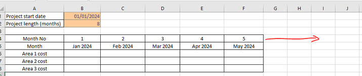
I am making a project cost forecasting sheet and want to be able to hide (or populate, whichever is easier) columns based on how long the project will run for
- Enter start date of project (01/01/2024)
- Enter project length in months (say 14 months)
- Formula should hide (or populate) columns up until column J (which is 8 months)

I could frig around with lots of IF commands and conditional formatting but wondering if there is neat solution?
Thanks

 

[kevin9999]

Please update your profile so helpers can see what version of Excel you're using (solutions will vary).
Assuming you're using 365/2021 then the following should give you what you want:

Book1
	A	B	C	D	E	F	G	H	I	J
1	Project start date	1/01/2024
2	Project length (months)	8
3
4	Month No	1	2	3	4	5	6	7	8
5	Month	Jan 2024	Feb 2024	Mar 2024	Apr 2024	May 2024	Jun 2024	Jul 2024	Aug 2024
6	Area 1 Cost
7	Area 1 Cost
8	Area 1 Cost
9
Sheet1

Cell Formulas
Range	Formula
B4:I4	B4	=SEQUENCE(1,B2)
B5:I5	B5	=TEXT(DATE(YEAR(B1),SEQUENCE(1,B2),1),"mmm yyyy")
Dynamic array formulas.

Cells with Conditional Formatting
Cell	Condition		Cell Format	Stop If True
A4:M18	Expression	=AND($A4<>"",A$4<>"")	text	NO

 

[Peter_SSs]

Or perhaps this? (Col I not Col J?)
Format row 5 as "mmm yyyy"
Also assuming recent version with relevant functions.

24 02 21.xlsm
	A	B	C	D	E	F	G	H	I	J
1	Project start date	1/01/2024
2	Project length (months)	8
3
4	Month No	1	2	3	4	5	6	7	8
5	Month	Jan 2024	Feb 2024	Mar 2024	Apr 2024	May 2024	Jun 2024	Jul 2024	Aug 2024
Project run

Cell Formulas
Range	Formula
B4:I4	B4	=SEQUENCE(,B2)
B5:I5	B5	=EDATE(B1,B4#-1)
Dynamic array formulas.

 

[Peter_SSs]

Oops, I forgot the formatting.

24 02 21.xlsm
	A	B	C	D	E	F	G	H	I	J	K
1	Project start date	1/01/2024
2	Project length (months)	8
3
4	Month No	1	2	3	4	5	6	7	8
5	Month	Jan 2024	Feb 2024	Mar 2024	Apr 2024	May 2024	Jun 2024	Jul 2024	Aug 2024
6	Area 1 Cost
7	Area 1 Cost
8	Area 1 Cost
9
10
Project run

Cell Formulas
Range	Formula
B4:I4	B4	=SEQUENCE(,B2)
B5:I5	B5	=EDATE(B1,B4#-1)
Dynamic array formulas.

Cells with Conditional Formatting
Cell	Condition		Cell Format	Stop If True
A4:T8	Expression	=COLUMNS($A:A)<=$B$2+1	text	NO

 

[kanemitchell99]

Please update your profile so helpers can see what version of Excel you're using (solutions will vary).
Assuming you're using 365/2021 then the following should give you what you want:

Book1
	A	B	C	D	E	F	G	H	I	J
1	Project start date	1/01/2024
2	Project length (months)	8
3
4	Month No	1	2	3	4	5	6	7	8
5	Month	Jan 2024	Feb 2024	Mar 2024	Apr 2024	May 2024	Jun 2024	Jul 2024	Aug 2024
6	Area 1 Cost
7	Area 1 Cost
8	Area 1 Cost
9
Sheet1

Cell Formulas
Range	Formula
B4:I4	B4	=SEQUENCE(1,B2)
B5:I5	B5	=TEXT(DATE(YEAR(B1),SEQUENCE(1,B2),1),"mmm yyyy")
Dynamic array formulas.

Cells with Conditional Formatting
Cell	Condition		Cell Format	Stop If True
A4:M18	Expression	=AND($A4<>"",A$4<>"")	text	NO

Wow thank you I haven't come across the sequence function before that is brilliant!!

 

[kevin9999]

Glad we could help, and thanks for the feedback

 

[Peter_SSs]

Glad you got a successful outcome.

Clearly it means that you do have a recent version of Excel. It would be very helpful for the future if you did update your profile (as requested above) so we know which recent version and so that information is always available.
Click your user name at the top right of the forum, then ‘Account details’. Don’t forget to scroll down & ‘Save’ after you have entered the relevant information.

If your version is 365 then you can also get both rows of results with a single formula in cell B4.

24 02 21.xlsm
	A	B	C	D	E	F	G	H	I	J
1	Project start date	1/01/2024
2	Project length (months)	8
3
4	Month No	1	2	3	4	5	6	7	8
5	Month	Jan 2024	Feb 2024	Mar 2024	Apr 2024	May 2024	Jun 2024	Jul 2024	Aug 2024
6	Area 1 Cost
7	Area 1 Cost
8	Area 1 Cost
Project run (2)

Cell Formulas
Range	Formula
B4:I5	B4	=LET(s,SEQUENCE(,B2),VSTACK(s,EDATE(B1,s-1)))
Dynamic array formulas.

Cells with Conditional Formatting
Cell	Condition		Cell Format	Stop If True
A4:T8	Expression	=COLUMNS($A:A)<=$B$2+1	text	NO