Horizontal Filters

[tinferns]

Hello Team,
Firstly thanks a million for all your help in the past.

I need your help on the below:

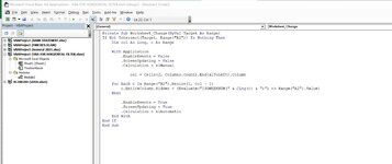
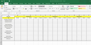
I prefer formula(s), but I guess this will work best with a VBA. In the below table, I want to apply a horizontal filter based on Week Number. So If I have selected Week 41, I want to see all 6 departments' dates between 05Oct2020 - 09Oct2020. Rest has to be hidden.

If required can place another table in the file to help VBA choose START DATE & END DATE depending on Year and Week Number. The format I am working is shown below:

VBA FOR HORIZONTAL FILTER.xlsx
	A	B	C	D	E	F	G	H	I	J	K	L	M	N	O	P	Q	R	S	T	U	V	W	X	Y	Z	AA	AB	AC	AD	AE	AF	AG	AH	AI	AJ	AK	AL	AM	AN	AO	AP	AQ	AR	AS	AT	AU	AV	AW	AX	AY	AZ	BA	BB	BC	BD	BE	BF	BG	BH	BI
1	Week No	Department 1					Department 2					Department 3					Department 4					Department 5					Department 6					Department 1					Department 2					Department 3					Department 4					Department 5					Department 6
2	41	05-Oct	06-Oct	07-Oct	08-Oct	09-Oct	05-Oct	06-Oct	07-Oct	08-Oct	09-Oct	05-Oct	06-Oct	07-Oct	08-Oct	09-Oct	05-Oct	06-Oct	07-Oct	08-Oct	09-Oct	05-Oct	06-Oct	07-Oct	08-Oct	09-Oct	05-Oct	06-Oct	07-Oct	08-Oct	09-Oct	12-Oct	13-Oct	14-Oct	15-Oct	16-Oct	12-Oct	13-Oct	14-Oct	15-Oct	16-Oct	12-Oct	13-Oct	14-Oct	15-Oct	16-Oct	12-Oct	13-Oct	14-Oct	15-Oct	16-Oct	12-Oct	13-Oct	14-Oct	15-Oct	16-Oct	12-Oct	13-Oct	14-Oct	15-Oct	16-Oct
3	Number of Emplooyes
4	Employees Present
5	Employees Absent
6
7	Total Productivity
8	Expected Productivity
9	Actual Producitivty
10	Difference
11
12	Quality Scores
13	Expected QA Scores
14	Difference
15
16	Client Scores
17	Expected Client Scores
18	Difference
19
Sheet1

Start Date and End Date based on Year and Week Number (I can keep this table hidden somewhere in the sheet)

VBA FOR HORIZONTAL FILTER.xlsx
	A	B	C	D
21	Year	Week No	Start Date	End Date
22	2020	41	5-Oct-20	9-Oct-20
23	2020	42	12-Oct-20	16-Oct-20
24	2020	43	19-Oct-20	23-Oct-20
25	2020	44	26-Oct-20	30-Oct-20
26	2020	45	2-Nov-20	6-Nov-20
27	2020	46	9-Nov-20	13-Nov-20
28	2020	47	16-Nov-20	20-Nov-20
29	2020	48	23-Nov-20	27-Nov-20
30	2020	49	30-Nov-20	4-Dec-20
31	2020	50	7-Dec-20	11-Dec-20
32	2020	51	14-Dec-20	18-Dec-20
33	2020	52	21-Dec-20	25-Dec-20
34	2020	53	28-Dec-20	1-Jan-21
35	2021	1	4-Jan-21	8-Jan-21
36	2021	2	11-Jan-21	15-Jan-21
37	2021	3	18-Jan-21	22-Jan-21
38	2021	4	25-Jan-21	29-Jan-21
39	2021	5	1-Feb-21	5-Feb-21
40	2021	6	8-Feb-21	12-Feb-21
41	2021	7	15-Feb-21	19-Feb-21
42	2021	8	22-Feb-21	26-Feb-21
43	2021	9	1-Mar-21	5-Mar-21
44	2021	10	8-Mar-21	12-Mar-21
45	2021	11	15-Mar-21	19-Mar-21
46	2021	12	22-Mar-21	26-Mar-21
47	2021	13	29-Mar-21	2-Apr-21
48	2021	14	5-Apr-21	9-Apr-21
49	2021	15	12-Apr-21	16-Apr-21
50	2021	16	19-Apr-21	23-Apr-21
51	2021	17	26-Apr-21	30-Apr-21
52	2021	18	3-May-21	7-May-21
53	2021	19	10-May-21	14-May-21
54	2021	20	17-May-21	21-May-21
55	2021	21	24-May-21	28-May-21
56	2021	22	31-May-21	4-Jun-21
57	2021	23	7-Jun-21	11-Jun-21
58	2021	24	14-Jun-21	18-Jun-21
59	2021	25	21-Jun-21	25-Jun-21
60	2021	26	28-Jun-21	2-Jul-21
61	2021	27	5-Jul-21	9-Jul-21
62	2021	28	12-Jul-21	16-Jul-21
63	2021	29	19-Jul-21	23-Jul-21
64	2021	30	26-Jul-21	30-Jul-21
65	2021	31	2-Aug-21	6-Aug-21
66	2021	32	9-Aug-21	13-Aug-21
67	2021	33	16-Aug-21	20-Aug-21
68	2021	34	23-Aug-21	27-Aug-21
69	2021	35	30-Aug-21	3-Sep-21
70	2021	36	6-Sep-21	10-Sep-21
71	2021	37	13-Sep-21	17-Sep-21
72	2021	38	20-Sep-21	24-Sep-21
73	2021	39	27-Sep-21	1-Oct-21
74	2021	40	4-Oct-21	8-Oct-21
75	2021	41	11-Oct-21	15-Oct-21
76	2021	42	18-Oct-21	22-Oct-21
77	2021	43	25-Oct-21	29-Oct-21
78	2021	44	1-Nov-21	5-Nov-21
79	2021	45	8-Nov-21	12-Nov-21
80	2021	46	15-Nov-21	19-Nov-21
81	2021	47	22-Nov-21	26-Nov-21
82	2021	48	29-Nov-21	3-Dec-21
83	2021	49	6-Dec-21	10-Dec-21
84	2021	50	13-Dec-21	17-Dec-21
85	2021	51	20-Dec-21	24-Dec-21
86	2021	52	27-Dec-21	31-Dec-21
87	2022	1	3-Jan-22	7-Jan-22
88	2022	2	10-Jan-22	14-Jan-22
Sheet1

Cell Formulas
Range	Formula
C22:C88	C22	=DATE(A22,1,-2)-WEEKDAY(DATE(A22,1,3))+B22*7
D22:D88	D22	=DATE(A22, 1, -2) - WEEKDAY(DATE(A22, 1, 3)) + B22 * 7 + 4

 

[jasonb75]

I don't see where filtering fits into the question.

In B2, then drag right.

=VLOOKUP($A$2,Table1[[Week No]:[Start Date]],2,0)+MOD(COLUMNS($B$2:B$2)-1,5)

I've assumed that your table is named 'Table1', if it is different then you will need to change it.

Alternatively, you could just use the first part of the formula in B2.

=VLOOKUP($A$2,Table1[[Week No]:[Start Date]],2,0)

Then enter

=B2+1

into C2 and drag that right as far as F2. Finally, enter

=B2

into G2 and drag that right as far as needed.

The first method is simpler to set up, the second uses simpler formulas and is more efficient, although the difference would be negligible.

 

[tinferns]

Hi Jason.. Thanks for your super quick reply. The above formula gives me the dates based on week number.. thanks for that.

I want the formula or vba to hide & unhide columns.

For Eg. I have updated or I am looking for data only for Week Number 41 in the above example. This has to

UNHIDE: Column B - Column AE = Week 41
HIDE: Column AF to Column BI = Week 42

I am sorry I did not explain the scenario clearly earlier. Hope the above explanation is clear.

Thanks..

 

[jasonb75]

My fault for not scrolling right far enough, if I had then I would have seen it Because I wasn't seeing the relevance of the filter, I incorrectly thought that you were trying to fill the dates.

You can't filter in place with formulas, at best you can reproduce the relevant data in a different sheet. (Easier with office 365 but still possible with older versions).

The other option is to hide / unhide the columns on the existing sheet based on the week number using vba.

Which would you prefer?

 

[tinferns]

Thanks Jason..

I am using O 365 and 2019.

I will stick to VBA for now.

Please send me the script.

Thanks in advance..

 

[jasonb75]

Try this in the worksheet module (select the sheet, then right click the tab and 'view code'. This will run automatically when you change the week number in A2.
The additional table for the week numbers is not required.

Private Sub Worksheet_Change(ByVal Target As Range)
If Not Intersect(Target, Range("A2")) Is Nothing Then
    Dim col As Long, c As Range
    
    With Application
        .EnableEvents = False
        .ScreenUpdating = False
        .Calculation = xlManual
        
            col = Cells(2, Columns.Count).End(xlToLeft).Column
    
    For Each c In Range("B2").Resize(1, col - 1)
        c.EntireColumn.Hidden = (Evaluate("ISOWEEKNUM(" & CLng(c) & ")") <> Range("A2").Value)
    Next
    
        .EnableEvents = True
        .ScreenUpdating = True
        .Calculation = xlAutomatic
    End With
End If
End Sub

 

[tinferns]

Hi Jason,
Thanks for sending the code so quickly. I have pasted the code exactly how you have instructed, however when I change the week in A2 no action is visible.

I changed the week number to 42, thus Column B to AE should have hidden. Nothing happened. I guess I am not doing something right..

Screenshots attached.

Please help.

Thanks.

 

[jasonb75]

You have put the code into a general module, not the worksheet module.

Try this in the worksheet module (select the sheet, then right click the tab and 'view code'.

If you had done this then it would have taken you directly to the correct module, which is the one named Sheet1 (Sheet1) in your first screen capture.

 

[tinferns]

Hi Jason .. thanks for your reply.. I guess I am doing it right now. when I change to 42 all the columns are getting hidden and when I change back to 41, getting the below Debug error.

Private Sub Worksheet_Change(ByVal Target As Range)
If Not Intersect(Target, Range("A2")) Is Nothing Then
Dim col As Long, c As Range

With Application
.EnableEvents = False
.ScreenUpdating = False
.Calculation = xlManual

col = Cells(2, Columns.Count).End(xlToLeft).Column

For Each c In Range("B2").Resize(1, col - 1)
c.EntireColumn.Hidden = (Evaluate("ISOWEEKNUM(" & CLng(c) & ")") <> Range("A2").Value)
Next

.EnableEvents = True
.ScreenUpdating = True
.Calculation = xlAutomatic
End With
End If
End Sub

 

[jasonb75]

Try this way instead, it appears that the first method doesn't pick up the hidden columns to the right of the last visible column.
You will probably have to close excel and reopen it for this to work as the code would have ended with events being disabled.

Private Sub Worksheet_Change(ByVal Target As Range)
If Not Intersect(Target, Range("A2")) Is Nothing Then
    Dim col As Long, c As Range
    
    With Application
        .EnableEvents = False
        .ScreenUpdating = False
        .Calculation = xlManual
        
            cols = UsedRange.Columns.Count
    
    For Each c In Range("B2").Resize(1, cols - 1)
        c.EntireColumn.Hidden = (Evaluate("ISOWEEKNUM(" & CLng(c) & ")") <> Range("A2").Value)
    Next
    
        .EnableEvents = True
        .ScreenUpdating = True
        .Calculation = xlAutomatic
    End With
End If
End Sub