How do I do a sum using cell colours and data in it.

[ghrek]

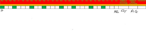
I have a workbook and in row 2 between columns D and AE there are some cells that are blank, some that are coloured green and some will be red with the word NO.

What im trying to do is in column AG is input a number for any cells that change colour. If any of the cells that are coloured green in that row change to red and the word NO is put in it I need the number in column AG for that row increased by one and obviously if turned back to green I need it reduced.

How do I do that?

Thanks

 

[Beneindias]

Hi,

You can create a Macro to give you the code of the background color.

Function GetBackgroundColor(cell As Range)    
GetBackgroundColor = cell.Interior.Color 
End Function

Then, you just need to create an helper column and past the function, referencing the cell.
(for this example, i'm assuming that you have your colors in column A, and your helper will be column B)

in cell B1, you put:

=GetBackgroundColor(A1)

Now, in column B, you will have the code of the background color.

From here, you just need to do some IF functions, and you have your problem solved.

Hope it helps

 

[ghrek]

Sorry think I might of confused you.

In columns A & B there is other data and I need that left alone. Apologies on the state of it but if you look at attachment what I mean is if I change any of the cells between column D and AE that are coloured GREEN to red and input NO I need the number in column AG increasing or decreasing depending on what I do.

 

[Fluff]

How about

=countifs(D2:AE2,"No")

 

[ghrek]

Brill Fluff just waht I needed

 

[Fluff]

Glad we could help & thanks for the feedback.

 

[Fluff]

In future please mark the post that contains the solution, not your post saying it works, I have changed it for you this time.
Thanks

 

[ghrek]

In future please mark the post that contains the solution, not your post saying it works, I have changed it for you this time.
Thanks

oopppssss sorry

 

[ghrek]

Sorry I just realised I need to do it a different way

In column AF I need to put in the number of collections planned and if I turn one of the cells to red and put NO in I need the value reducing by one.

As per attachment earlier there at present there are 8 collections and this would be put in column AF but as stated if I change any then I need that reducing to 7 etc etc etc depending on how many I change.

 

[Fluff]

How about

=8-countifs(D2:AE2,"No")