How to copy looked up data from one workbook to looked up ranges in another workbook

HarryFröhlich

Board Regular
Joined
Mar 25, 2003
Messages
116
Hi everybody!

I would like to pick your brains, please...

The background: At the end of each month, consultants provide me with a spreadsheet that contains the following data in columns:

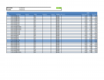
1. The name of the client for whom they did work on any given/specific day (let's assume the name is typed in column A). If a consultant saw the client on the 2nd, 10th and 23rd of a month, it follows that the name of the client will show 3 times. If he saw another client 5 times, the client's name will show 5 times etc. Any one or all of 30 clients may be seen.
2. The number of hours that they spent with the client (let's assume that this is indicated in column B)
3. And lastly, whether the hours spent with the client is billable or non-billable. (let's assume that this is indicated in column C)

An example:
Workbook name = "Peter time sheet data March 2020.xlsx"
A1 (Heading)= Client name
B1 (Heading)=Hours spent
C1 (Heading)=Billable or Non-Billable

Actual data:
A2 = ABC
B2 = 1.5
C= Billable

There are 20 consultants who provide me with their time sheets...

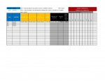
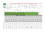
At the end of the month in question, I have to calculate the billable and non-billable hours spent with each client for each of the consultants and then carry these hours over to a separate recon workbook for each consultant and for each client. Let's call this workbook "Recon workbook March 2020.xlsx". This workbook summarises the time that each of the 20 consultants spent with each of the 30 clients. The names of the consultants appear below one another in rows down column A while the names of the 30 clients appear in columns B, C, D etc... Let's assume Peter's name shows in cell A7 and client ABC in column C.

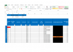
What I currently do is to to open a workbook of a consultant (let's assume that I start with Peter's workbook above). I then use a filter in column A to pick each client one by one in column A. In my Example let's assume that client ABC shows up 3 times. All other clients will be hidden. I now check if the hours are billable or non-billable. I then filter for that if some are billable and some are not. Let's assume all are billable. Once that is done, I highlight the hours in column B with my mouse and look at the right lower section of Excel what the Sum value of the highlighted range is. I then write this value down and copy these hours to the recon workbook. In my example above, the hours that Peter had spent with client ABC will be entered in cell C7.

I am really hopeful that someone will be able to help me automate this tedious task with VBA...

To summarise,

1. there are 20 consultants whose workbooks all have different names to identify their own time sheets (say peter)
2. each consultant's workbook changes with the name of the new month for which the hours are captured (say March 2020)
3. Each consultant's workbook only includes data of a single month
4. Each workbook could include time spent with a single client or up to 30 clients and the time spent for each client has to be calculated from the spreadsheet
5. The values for each consultant is to be carried over to the recon spreadsheet (for the relevant month, say March) for each respective client. If Peter saw 5 clients (ABC 19 hours, BCD 26 hours, CDE 27 hours, DEF 28 hours and EFG 29.5 hours), the hours spent with each client has to be transferred to each corresponding column in the recon spreadsheet against Peter's name in the recon spreadsheet.

Did I make sense? hehe I really hope so...

And I also hope someone will come up with a great plan!

Kind regards

Harry
 

Excel Facts

Round to nearest half hour?
Use =MROUND(A2,"0:30") to round to nearest half hour. Use =CEILING(A2,"0:30") to round to next half hour.
For each month I would amalgamate all of the data from all of the consultants into one workbook. Having a master
workbook covering all months would be a good idea too.

I would use Column A to hold the consultants name.

You did not mention that you hold the date of the consultation. If you do suggest that this is in column B.

So :

A - Consultants name
B - Consultation date
C - Clients name
D - Hours
E - Billable or Non-Billable

What happens if two clients have the same name?
Is the client identified by their name and not a reference number?
If the former is the case then is it likely that the name will be written in different ways thereby appearing to be a different client.

Is it essentail that the recon workbook lists clients horizontally rather than vertically as the latter would be much easier to manage.

Is the above possible?

If so then the first step is to amalgamate the workbooks so that you just have the data in one table.

Let me know and then I can help you more.
 
Upvote 0
Hi there HighAndWilder!

Cool nickname... ;)

Thanks for the reply! Greatly appreciated, thanks. Just this morning I thought that I should probably break my post/request down into more manageable chunks by asking questions based on steps that I was thinking of using.... And then you posted....

Please allow me to initially answer your questions with a broad brush before answering each more specifically.

Each consultant has a monthly spreadsheet that runs from the first day of the month and ends on the last day, weekends included. The spreadsheet shows the actual date (e.g. 01/03/2020 for the first of March 2020) in column A and that it is a Sunday in column B. Please accept my apologies for buggering up the column detail of my initial post. The actual days in the consultant's summary for March is relevant on his personal level, but for the summarised workbook, all that is needed is the total hours spent with a client through the course of the full month.

That is why I did not mention days etc.

You are absolutely correct, though, in that more detail regarding dates etc is available in the consultant's workbook. It is just that those detail is irrelevant as far as I can see, but if you think that it is, then I am open to why you think so.

What I thought of doing is the following:

Step 1: Open a consultant's workbook.
Step 2a: Do an Advanced Filter to determine the unique names of clients seen through the month in the client column and
Step 2b: Copy the unique names to another section of the worksheet. Let's say that the unique names will be placed in column O from O2 down
Step 3: Use SUMIFS in column P, starting at P2, to sum the total billable (the two required criteria in the SUMIFS function in this case) hours for each unique client in column O, using the hours in the main spreadsheet as sum range. The heading in O1 is simply "Client", in P1 it is "Billable" and in Q1 it is "Non-billable"
Step 4: Use the same SUMIFS function in column Q, starting at Q2 to determine the hours spent at a client for non-billable hours.

As an aside: The spreadsheet that the consultant uses calculates the hours spent at each client by asking for a start time in a column (J) and an end time in another column (K), say 10h00 start and 11h30 end. The total time spent is calculated in column I. If the values in column O is formatted as TIME, then SUMIF / SUMIFS does not calculate the sum correctly. The values in I has to be shown as numbers by Subtracting the Start Time from the End Time and multiplying the answer by 24 or by using the more involved HOUR, MINUTE and SECOND function. The first is much easier.

Anyway, I was thinking of doing steps 1 through 4 above for each consultant and to record some VBA code to do this.

So, even if Peter spent 22 days with Client ABC, the specific days and time frames that he'd spent with the client are not relevant. I only need to know that he'd spent 42 hours in total with Client ABC during the month, for 42 hours will be carried over to the summary spreadsheet.

Once the total billable and non-billable hours for a consultant is calculated and summarised in the consultant's own spreadsheet with the 4 steps above, I then embark on transferring these values to the spreadsheet which summarises all the hours (both billable and non-billable in separate cells) spent with each client for the given month.

This is where my problem lies - how can I automate this process...

This is the manual process:

The consultant's name is already shown in the summary sheet as one of 20 (say...) in column A. Transferring hours spent manually requires me to look for the consultant's name in column A until I find Peter in A7 (say...) and then to scroll to the right until I find Client ABC in a column (say column R) and to enter the value of 42 (calculated) in Cell R7. If Peter also saw Client BCD for 22.5 hours, I'd find client BCD in column F (say...) and enter the figure 22.5 in cell F7 against Peter's name. I will do this until all the clients that Peter had seen have been accounted for. All non-billable hours spent with any client are added together and entered in cell B7 and is only used to ensure that the total hours worked by Peter in his own spreadsheet checks with the hours carried over to the summarised spreadsheet.

The process is repeated for all the other consultants. If another consultant also worked with Client ABC and this other consultant's name is registered in A2, then the hours that consultant A2 had spent with Client ABC will just be captured in R2, for Client ABC "occupies" column R.

I was thinking of placing all the consultant's workbooks and the summary workbook in the same folder and then to run a macro to transfer the values from each consultant;s workbook to the summary workbook by running a macro (after having run steps 1 to 4 above) that should ask me to provide it with the target workbook's name (which I could simply call a.xlsx or A.xlsm for simplicity until all data is carried over and then rename it) to transfer the data to the relevant fields using VLOOKUP, MATCH or whatever is required... hehe - discombobulating myself... I don't even need others to do it! hehe

The problem that I have is that there is a "system" and a "structure" already in place and the man in charge simply wants the data to be carried over without making changes to the "structure". So, data in columns have to remain there - cannot be switched to rows - and vice versa. The "summary" workbook is used to prepare invoices and to bill the clients at the hourly rates that each consultant charges while the data captured in each consultant's workbook is printed as PDFs and attached to the invoices sent to the clients.

The workbooks that each consultant uses is also pre-populated with the names of the clients and they may only pick these names from drop down lists in their workbooks. There is, therefore, no fear of inconsistency in the way names are spelled or abbreviated.

A summary for each consultant in a single workbook is something that I will be working on at a later date. The data for each consultant is printed out and saved as PDFs for each month at the moment and is sufficient.

Please accept my apologies for the long post HighAndWilder.

My problem seems to start after step 4...

Hope all my explanation helps!

Harry
 
Upvote 0
Hi Harry

I've got some time to help you on this one.

Lets do it step by step.

I can provide some basic code in a master workbook that will open each workbook in a specified folder and produce a
unique list of clients in another specified workbook / sheet. It will then, for each of these clients, calculate the summary information.

Are you able to post an image of the spreadsheet from the consultants and the spreadsheet that you are trying to produce so I can look at the next steps.
 
Upvote 0
Great! Thank you!

I attach two images:
The first should provide enough information as far as the structure of the current sheet completed by each consultant. This excludes my Advanced Filtering, SUMIFS etc
The second is the sheet into which all the data has to be transferred into. No transfer of hours per client is included in the attached image Recon March 2020

Both spreadsheets have to retain this structure.

Thanks again!

h
 

Attachments

  • Peter March 2020.png
    Peter March 2020.png
    48.2 KB · Views: 11
  • Recon March 2020.png
    Recon March 2020.png
    31.3 KB · Views: 11
Upvote 0
O, by the way, I am not actually trying to produce the second spreadsheet from the consultants' data- the data of each consultant simply has to be transferred into an existing spreadsheet that has a standard template, if you will... This is the one called Recon March 2020.PNG. A new one is created for each month, and is easier done by simply clearing all the fields that do not contain formulas in a current one and renaming it for the new month. Would you agree?
 
Upvote 0
Hi HarryFrohlich

I have developed some code which takes the data from the individual consultants workbooks and combines it into one
temporary worksheet. At the moment it takes ALL workbooks placed in a single folder selected by the user when they run the code.
I suggest that each months workbooks are stored together in one folder.

Question: Where does the consultants name come from, the file name?

Question: Where does the month come from? It can come from one of the entries in the date column
if not available from elsewhere. It could also come from name of the folder containing the files.

Question : When the horizontal list of clients is written to the summary worksheet do the names need to be in alphabetical order?
If not then what order? The default is the order in which it finds them in the source data.

Awaiting your response to these questions.

I'll make some changes if appropriate and then send you some code to check out.

Take care and stay safe.
 
Upvote 0
That is great, HighAndWilder!

The answer to your questions regarding the names of the consultants: yip, the file for a given month identifies each consultant's file by using his/her name and the name of the month and year, e.g. Peter March 2020, Tom March 2020.

The names of the consultants are pre-populated in the summary file. If a consultant did not submit a workbook, then that consultant will show as outstanding until the workbook is submitted, when data is carried over to the summary file. This means that, if there are 20 consultants and 15 have submitted their files for me to place in the same folder that you mention, then the temporary file may only summarise the data of the 15, but the FINAL destination file will still require the data of all 20 consultants to be entered.

Will the code allow for it to be run again a day or what later, if the outstanding files have been received and placed in the folder after the code had been run with only some files in the folder the first time? If a consultant had made a mistake with his/her file and then sent in a corrected file, can the code be run again to update the transferred data?

The name of the month can come from wherever best suits you. If this is to be used to name the destination file, it must be said that the name of the final destination file can be changed to whatever is required anyway after whatever code has run anyway, not so? So I wouldn't bother too much with this. The names of the consultants are important, as are the names of the clients that each consultant billed hours to. These must match perfectly, as you'd alluded to before. A spelling mistake in the name of a consultant in the file name for a given month will not find a match in the final destination file (The name Petr in the file name Petr March 2020.xlsx will not find and match the required name of consultant Peter in the final summary file, e.g.).

The names of the clients are in alphabetical order, but the list may expand or contract. The list in the FINAL SUMMARY will be pre-populated in alphabetical order and will always include all the names of all the clients, whether any consultant billed any hours to a client or not. If no consultant had spent time with a specific client in March, for example, then the summary will show zero billable hours against that client for the month. The source data will differ for each consultant. Peter may see 5 specific clients while Tom may see one of them and 7 others...

Thanks again HighAndWilder. I truly appreciate the help! I tried using MATCH and INDEX last night but then realised that I need something like that to pinpoint an intersection for, say, Peter and client A, and then to write something copied from the Peter workbook or your temporary workbook into that intersection for each client that Peter had seen... Still trying to figure out a solution! hehe... Glad you are spending time on it!

Looking forward to your response!

Harry
 
Upvote 0
Hi Harry

Thanks for the last message.

Can I suggest that the FINAL SUMMARY worksheet does not have the consultants and clients pre-populated

It is always best and easiest to report on what one finds in the source data so I suggest this:

That the source data is amalgamated (Note 1) and rows are added to this (Note 2) which represent dummy consultations for
those clients who did not see a consultant in the month and for those consultants who do not see a client in the month.
These rows are only used to avoid having to find which column the client appears in on the FINAL SUMMARY worksheet
and which row the consultant appears in. The adding of these rows to the amalgamated data will be automated and
clearly identified as dummy rows as the start time and end time of the consultationwill be the same resulting in zero duration

The amalgamated data is used in the SUMIFS formulas in the client columns. Either the amalgamated data worksheet can
be hidden (suggested) or the results of the formulas in the client columns can be changed to just the value of the
result an the amalgamated data worksheet not included in the FINAL SUMMARY workbook.
No decision is required on this last point yet as it does not involve a lot of coding.

What will be required is a worksheet containing a list of all clients. I am sure that you already have one. I'll create a dummy one for
testing purposes. If this worksheet is called 'Clients' and has just one column with a heading of 'Client'.

Do the consultants have to appear in any particular order.

Note 1 : This is what I am doing already in the step by step approach.

Note 2 : I have not done this bit yet but maybe tonight if a better offer does not come my way.

I will hopefully post some code for you tomorrow that you can test and comment on.

If, as you mentioned earlier, consultants do not submit their workbooks, all you have to do is add the workbook
to the folder for the month and run the code again. It will produce the FINAL SUMMARY workbook from scratch.
This is nearly always an easier way to do things like this.

HighAndWilder

P.S. The name comes from my love of mountains in bad weather. The only thing that I can climb at the moment
is the stairs!!
 
Upvote 0
Hi there again!

I'd actually looked at your profile to see whether you had your name available and noticed that you live in a stunning area - The Jurassic Coast. Incredibly beautiful, I see. No wonder you love the outdoors, and mountains and wild weather in particular. You probably do mountain biking as well?

Anyway...

I am getting somewhat concerned that all your help may end up being for nothing because I have to have the data in a very strict format. If it were up to me I's probably use the end of what you come up with to achieve what the powers that be require, but even sorting the consultants alphabetically in the final workbook is a no-no... They have to run from first employed to last employed / contracted...

Because of this, I deleted the confidential information from the ACTUAL FINAL workbook (the one I'd previously submitted a picture of, but then without the column and the row headers and only a small section of) and now upload a series of pictures that cover the whole worksheet from column A tot BF. I only included the first number of rows (which hold the consultants' data), but the rows go down to 47 in the actual worksheet.

Please take a look at this sheet, because the FINAL worksheet has to be exactly like this...

In this sheet, certain fields contain data that is pre-populated. These are the columns B to K, with the first name of the consultant in C
Data carried over from each consultant's workbook is placed in the row linked to the consultant in columns L, M, N, P and range T:BC
There are a number of formulas in the sheet. Column O=L+M+N, Q=P-O, R=L-BD and BD=SUM(T:BC)
Column S gets data from elsewhere and is of no consequence here.

I will also upload a series of pictures from a consultant's workbook in a seperate post.

I hope this does not upset the apple cart too much...

h
 

Attachments

  • Final spreadsheet columns A to K.png
    Final spreadsheet columns A to K.png
    129.5 KB · Views: 11
  • Final spreadsheet columns AE to AV.png
    Final spreadsheet columns AE to AV.png
    54 KB · Views: 11
  • Final spreadsheet columns AV to BF.png
    Final spreadsheet columns AV to BF.png
    42 KB · Views: 10
  • Final spreadsheet columns K to Q.png
    Final spreadsheet columns K to Q.png
    51.3 KB · Views: 11
  • Final spreadsheet columns Q to AE.png
    Final spreadsheet columns Q to AE.png
    55.1 KB · Views: 10
Upvote 0

Forum statistics

Threads
1,215,493
Messages
6,125,131
Members
449,206
Latest member
burgsrus

We've detected that you are using an adblocker.

We have a great community of people providing Excel help here, but the hosting costs are enormous. You can help keep this site running by allowing ads on MrExcel.com.
Allow Ads at MrExcel

Which adblocker are you using?

Disable AdBlock

Follow these easy steps to disable AdBlock

1)Click on the icon in the browser’s toolbar.
2)Click on the icon in the browser’s toolbar.
2)Click on the "Pause on this site" option.
Go back

Disable AdBlock Plus

Follow these easy steps to disable AdBlock Plus

1)Click on the icon in the browser’s toolbar.
2)Click on the toggle to disable it for "mrexcel.com".
Go back

Disable uBlock Origin

Follow these easy steps to disable uBlock Origin

1)Click on the icon in the browser’s toolbar.
2)Click on the "Power" button.
3)Click on the "Refresh" button.
Go back

Disable uBlock

Follow these easy steps to disable uBlock

1)Click on the icon in the browser’s toolbar.
2)Click on the "Power" button.
3)Click on the "Refresh" button.
Go back
Back
Top