How to make a dynamic horizontal line data range in excel?

linerangeguy

New Member
Joined
Jan 25, 2024
Messages
2
Office Version
  1. 365
Platform
  1. Windows
I have two data points, a low and a high. I want to create a line graph that recognizes these two points as a range. Then, I have a third data point which will be the only data point on the line (the only dot shown on this range line). The line itself will be showcasing the range between the low and high. The range line length should not matter as it will be the same length even if the low and high change (want to make this dynamic). Where the third point is will visually show where that data point is on that range (between the low and high data points).

So I would have a low, lets say 20, a high, lets say 69, and then a third data point, lets say 46. I want to make an excel line visual where it is dynamic to each of the figures (so if the low and highs change to lets say, 10 and 110, the line length will stay the same but will depict that new range). And then on this visual line, the 46 will be shown as a plot point on that line and will be dynamic (so if 46 changes to say, 78, then the dot positioning will change). Below is an example of what I'm trying to create in excel (and very bottom is the mini sheet).

1706203589220.png


And a follow up question would be how to incorporate this range within a cell. So looking at the image above, the "Low" "Range" High" and "Average" are all columns in excel with data points.

Thank you so much for your help in advance!

mrexcel line range question.xlsx
ABCD
3Data PointLowRangeHigh
4160155302
5218211261
6126126208
7209204374
85946128
9
10
11Data PointLowRangeHigh
12171164258
13140140231
149289187
15109109204
167777160
17
18
19Data PointLowRangeHigh
204024105
219992149
22148148227
239987160
249786142
25118112166
26105101172
27---
288374142
29131127176
30
31
32Data PointLowRangeHigh
33108103170
3411396177
359991143
369492167
37
38
39Data PointLowRangeHigh
40141136222
418180117
42128128241
43129121224
448777163
457670146
4610390175
Table
 

Excel Facts

Enter current date or time
Ctrl+: enters current time. Ctrl+; enters current date. Use Ctrl+: Ctrl+; Enter for current date & time.
Welcome to the MrExcel forum!

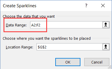
You've got a pretty big ask. I'm sure that you can get exactly what you want with some clever VBA programming, but it'll be a lot of work. Instead you might be able to use Sparklines, which is basically a mini-graph that fits in a single cell. Here's a link that explains a bit about them:


I played around a bit with them and came up with 2 options. Consider:

Spark.xlsx
ABCDEFGH
1Data PointLowRangeHigh
2159.93154.91301.9154.9083159.9283301.902
3218.19210.98261.05210.9788218.1876261.0514
4126.47126.47207.71126.4742126.4742207.713
5209.16204.01373.83204.0119209.1561373.826
658.68646.19128.3346.1903958.6858128.334
Sheet3
Cell Formulas
RangeFormula
F2:F6,H2:H6F2=B2
G2:G6G2=A2


Sparklines don't come across in XL2BB, but here's how it actually looks:

1706239329117.png


I placed the 3 points in the F:H columns. Then I clicked on the cell, went to the Insert Tab, and inserted a sparkline. I then gave it the F:H range, chose the Line type. I then clicked Markers to get the red dots, and changed the vertical axis to 0. The middle dot, your "data point" will always be exactly halfway through the graph, but the height will be relative to the end points.

Second option:

Spark.xlsx
ABCDEFGHI
9Data PointLowRangeHigh
10170.56164.18 #258.32164.182258.3172.032415
11139.7139.7 #230.87139.6964230.8670
12178.189.063 #187.489.0628187.40227.16227
13109.07108.75 #203.83108.749203.8270.102421
1412377.183 #159.5877.1831159.57716.68215
Sheet3
Cell Formulas
RangeFormula
F10:F14F10=B10
G10:G14G10=D10
C10:C14C10=REPT(" ",I10+15)&"#"
I10:I14I10=(A10-B10)/(D10-B10)*30


And how it actually looks:

1706239648108.png


I put the Low and High points in F:G, and a formula in I that calculates the distance that the data point will be from the low point. I then set up the Sparkline as before, using F:G as the range, and NOT clicking on Markers this time. Sparklines allow you to also put in a value in the cell. So I set the font in that cell to Consolas, which is a fixed pitch font, and changed the font size to 2. Which is very tiny! That allowed me to put 60 characters in the cell. The first 15 characters are before the line, then I used the distance formula from column I to figure out how many spaces to add, then I added a formula in column C. The cell is bolded, and I changed the font color to red. And if you change the value in column A, the red dot will automatically adjust.

So a couple of options! I hope one of them works for you. You can of course play around yourself with the other options and maybe come up with something more to your liking. Let us know how it works.
 
Upvote 0
ok got it - appreciate the detailed response and link! Went with the sparklines as an alternative and will brush up on my VBA. Thank you so much!!
Welcome to the MrExcel forum!

You've got a pretty big ask. I'm sure that you can get exactly what you want with some clever VBA programming, but it'll be a lot of work. Instead you might be able to use Sparklines, which is basically a mini-graph that fits in a single cell. Here's a link that explains a bit about them:


I played around a bit with them and came up with 2 options. Consider:

Spark.xlsx
ABCDEFGH
1Data PointLowRangeHigh
2159.93154.91301.9154.9083159.9283301.902
3218.19210.98261.05210.9788218.1876261.0514
4126.47126.47207.71126.4742126.4742207.713
5209.16204.01373.83204.0119209.1561373.826
658.68646.19128.3346.1903958.6858128.334
Sheet3
Cell Formulas
RangeFormula
F2:F6,H2:H6F2=B2
G2:G6G2=A2


Sparklines don't come across in XL2BB, but here's how it actually looks:

View attachment 105775

I placed the 3 points in the F:H columns. Then I clicked on the cell, went to the Insert Tab, and inserted a sparkline. I then gave it the F:H range, chose the Line type. I then clicked Markers to get the red dots, and changed the vertical axis to 0. The middle dot, your "data point" will always be exactly halfway through the graph, but the height will be relative to the end points.

Second option:

Spark.xlsx
ABCDEFGHI
9Data PointLowRangeHigh
10170.56164.18 #258.32164.182258.3172.032415
11139.7139.7 #230.87139.6964230.8670
12178.189.063 #187.489.0628187.40227.16227
13109.07108.75 #203.83108.749203.8270.102421
1412377.183 #159.5877.1831159.57716.68215
Sheet3
Cell Formulas
RangeFormula
F10:F14F10=B10
G10:G14G10=D10
C10:C14C10=REPT(" ",I10+15)&"#"
I10:I14I10=(A10-B10)/(D10-B10)*30


And how it actually looks:

View attachment 105776

I put the Low and High points in F:G, and a formula in I that calculates the distance that the data point will be from the low point. I then set up the Sparkline as before, using F:G as the range, and NOT clicking on Markers this time. Sparklines allow you to also put in a value in the cell. So I set the font in that cell to Consolas, which is a fixed pitch font, and changed the font size to 2. Which is very tiny! That allowed me to put 60 characters in the cell. The first 15 characters are before the line, then I used the distance formula from column I to figure out how many spaces to add, then I added a formula in column C. The cell is bolded, and I changed the font color to red. And if you change the value in column A, the red dot will automatically adjust.

So a couple of options! I hope one of them works for you. You can of course play around yourself with the other options and maybe come up with something more to your liking. Let us know how it works.
 
Upvote 0

Forum statistics

Threads
1,215,069
Messages
6,122,956
Members
449,096
Latest member
Anshu121

We've detected that you are using an adblocker.

We have a great community of people providing Excel help here, but the hosting costs are enormous. You can help keep this site running by allowing ads on MrExcel.com.
Allow Ads at MrExcel

Which adblocker are you using?

Disable AdBlock

Follow these easy steps to disable AdBlock

1)Click on the icon in the browser’s toolbar.
2)Click on the icon in the browser’s toolbar.
2)Click on the "Pause on this site" option.
Go back

Disable AdBlock Plus

Follow these easy steps to disable AdBlock Plus

1)Click on the icon in the browser’s toolbar.
2)Click on the toggle to disable it for "mrexcel.com".
Go back

Disable uBlock Origin

Follow these easy steps to disable uBlock Origin

1)Click on the icon in the browser’s toolbar.
2)Click on the "Power" button.
3)Click on the "Refresh" button.
Go back

Disable uBlock

Follow these easy steps to disable uBlock

1)Click on the icon in the browser’s toolbar.
2)Click on the "Power" button.
3)Click on the "Refresh" button.
Go back
Back
Top