How to sort by latest date in SUMPRODUCT

[lost_in_the_sauce]

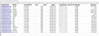
I have an array of sales data from multiple stores (180), and the data is entered by the stores at the end of each month. It all goes into an array. However, some stores will update their numbers, and in the array it adds a new line with a date/timestamp. For example, New York has 4 entries for February 2022, with different timestamps, and I only want the last one.

Currently I am using SUMPRODUCT like this:

=SUMPRODUCT((Data!$B$2:$B$1214=$B18)*(Data!$J$1:$P$1=C$2)*(Data!$F$2:$F$1214=$A18)*(Data!$J$2:$P$1214))

where $B18 is the month, C$2 is the $ category (sales, rent, etc), $A18 is the location, and $J:$2:$P$14 is the array of number values.

I have a column G with the timestamp. I've tried MAX but it looks like it pulls everything, I just want to add the condition for the latest date that also matches the other 3 conditions.

 

[awoohaw]

For someone to recreate your scenario requires a lot of thought and figuring out?
Can you help the forum help you by using the xl2bb add in and giving snapshot of the pertinent cells. There is a link to it below.
You can anonymize as necessary. You have Cell $B18 as a match value, but B2:B1214 is also a lookup range, which is okay, but it is confusing without seeing your worksheet. What is in cell $A18 (It is one of your lookup values)?

 

[awoohaw]

Is the the timestamp a complete date and time value? Is the month only a text expression? what is the max expression you are using, including the cell references (are there any non values in that range)?

 

[awoohaw]

Also, i think this portion is a typo: $J:$2:$P$14 is it supposed to be $J$2:$P$1214?

 

[lost_in_the_sauce]

For someone to recreate your scenario requires a lot of thought and figuring out?
Can you help the forum help you by using the xl2bb add in and giving snapshot of the pertinent cells. There is a link to it below.
You can anonymize as necessary. You have Cell $B18 as a match value, but B2:B1214 is also a lookup range, which is okay, but it is confusing without seeing your worksheet. What is in cell $A18 (It is one of your lookup values)?

Waiting on IT to see if I'll be allowed to add the extension on my work laptop.

>Also, i think this portion is a typo: $J:$2:$P$14 is it supposed to be $J$2:$P$1214?

Yep, that was a typo on my part. You are correct.

The attached image is a small bit of the array, but in this example I want the cell to pull the 4th entry for Feb Revenue for New York, which would be the 8th row, currently it pulls 5-8.

The timestamp is in format: 5/16/2022 6:03:57 PM or mm/dd/yy h:mm AM/PM under custom. There are no non values in the column.

 

[awoohaw]

Waiting on IT to see if I'll be allowed to add the extension on my work laptop.

>Also, i think this portion is a typo: $J:$2:$P$14 is it supposed to be $J$2:$P$1214?

Yep, that was a typo on my part. You are correct.

The attached image is a small bit of the array, but in this example I want the cell to pull the 4th entry for Feb Revenue for New York, which would be the 8th row, currently it pulls 5-8.

The timestamp is in format: 5/16/2022 6:03:57 PM or mm/dd/yy h:mm AM/PM under custom. There are no non values in the column.

i understand about IT issues!

 

[awoohaw]

can you post the text of the formula that is giving you problems?

 

[awoohaw]

How does this work:

Book1
	A	B	C	D	E	F	G	H	I	J
1		Month		Year		Name	Created Date			Revenue
2		January		2022		New York	2022-02-20 01:43			341,716.77
3		January		2022		New York	2022-05-16 17:59			0.00
4		January		2022		New York	2022-05-16 18:03			341,716.77
5		February		2022		New York	2022-03-10 14:21			533,074.54
6		February		2022		New York	2022-03-12 17:11			385,871.20
7		February		2022		New York	2022-05-16 18:00			0.00
8		February		2022		New York	2022-05-16 18:04			385,871.20
9		March		2022		New York	2022-04-11 14:20			494203.4
10		Apri		2022		New York	2022-05-17 17:17			412691.43
11		May		2022		New York	2022-06-11 18:12			275129.77
12
13
14		February	385871.2
Sheet1

Cell Formulas
Range	Formula
C14	C14	=SUM(((--(MAX((--(B14=$B$2:$B$11))*($G$2:$G$11))=$G$2:$G$11))*($J$2:$J$11)))

 

[lost_in_the_sauce]

How does this work:

Book1
	A	B	C	D	E	F	G	H	I	J
1		Month		Year		Name	Created Date			Revenue
2		January		2022		New York	2022-02-20 01:43			341,716.77
3		January		2022		New York	2022-05-16 17:59			0.00
4		January		2022		New York	2022-05-16 18:03			341,716.77
5		February		2022		New York	2022-03-10 14:21			533,074.54
6		February		2022		New York	2022-03-12 17:11			385,871.20
7		February		2022		New York	2022-05-16 18:00			0.00
8		February		2022		New York	2022-05-16 18:04			385,871.20
9		March		2022		New York	2022-04-11 14:20			494203.4
10		Apri		2022		New York	2022-05-17 17:17			412691.43
11		May		2022		New York	2022-06-11 18:12			275129.77
12
13
14		February	385871.2
Sheet1

Cell Formulas
Range	Formula
C14	C14	=SUM(((--(MAX((--(B14=$B$2:$B$11))*($G$2:$G$11))=$G$2:$G$11))*($J$2:$J$11)))

The formula =SUMPRODUCT((Data!$B$2:$B$1214=$B18)*(Data!$J$1:$P$1=C$2)*(Data!$F$2:$F$1214=$A18)*(Data!$J$2:$P$1214)) works great currently if the data is already cleaned up so that only the latest entry is in the array, but that's time consuming and I'm trying to make it easier going forward, so I'm trying to figure how to add to that formula to have it also select the MAX of the timestamps that satisfy the month, name, and revenue columns

 

[awoohaw]

I thought the formula in POST 8 does that. What am I missing?