HOW TO SPLIT PARTS OF TEXT STRING INTO 6 COLUMNS

JuicyMusic

Board Regular
Joined
Jun 13, 2020
Messages
210
Office Version
  1. 365
Platform
  1. Windows
I have tried and tried. I can adjust these types of formula's (somewhat) if I need to......but I just can't figure this one out.

Normal request: How to extract text after the last space in a string? I can do this.
Unusual: How to extract text after the space BEFORE the last space in a string. I CAN'T DO THIS ONE:(

In a nut shell.....I need to split a string into 6 parts, and these 6 parts going into a different column on the same row.
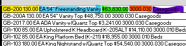
See the image I uploaded. The spacing or order of information is always constant and won't change.

Column C : Original String
See the 2nd image uploaded to see what type of text goes into column D thru I. See my red text where I explain. TYSM!!!!!


Here is a string for example.
GB-200 130.00 EA 54" Freestanding Vanity $63,830.00 3000.030 Casegoods
 

Attachments

  • Screenshot_split string into 6 columns by color.png
    Screenshot_split string into 6 columns by color.png
    6.5 KB · Views: 26
  • Screenshot_Data snapshot showing 6 columns.png
    Screenshot_Data snapshot showing 6 columns.png
    11.7 KB · Views: 26

Excel Facts

Can you AutoAverage in Excel?
There is a drop-down next to the AutoSum symbol. Open the drop-down to choose AVERAGE, COUNT, MAX, or MIN
Hi @JuicyMusic

Your data seems to be inconsistent at line 3 where there is no space between "GB-201" and "7.00".
Is that a typo?

If your data is inconsistent, it will be difficult to handle.
Meanwhile, here's a table with formulas that should work on your example string:

Book1.xlsm
CDEFGHI
1ORIGINAL TEXTHPGI CodeDescriptionCountTotal CostPH CodeType
2GB-200 130.00 EA 54" Freestanding Vanity $63,830.00 3000.030 CasegoodsGB-200 EA 54" Freestanding Vanity130.00$63,830.00 3000.030 Casegoods
Sheet35
Cell Formulas
RangeFormula
D2D2= LEFT(C2,FIND(" ",C2)-1)
E2E2= MID(C2,FIND(" ",C2,FIND(" ",C2)+1),FIND("~",SUBSTITUTE(C2," ","~",LEN(C2) - LEN( SUBSTITUTE(C2," ","") )-2))-FIND(" ",C2,FIND(" ",C2)+1))
F2F2= MID(C2,FIND(" ",C2)+1,FIND(" ",C2,FIND(" ",C2)+1)-FIND(" ",C2)-1)
G2G2= MID(C2,FIND("~",SUBSTITUTE(C2," ","~",LEN(C2) - LEN( SUBSTITUTE(C2," ","") )-2))+1,FIND("~",SUBSTITUTE(C2," ","~",LEN(C2) - LEN( SUBSTITUTE(C2," ","") )-1))-FIND("~",SUBSTITUTE(C2," ","~",LEN(C2) - LEN( SUBSTITUTE(C2," ","") )-2)))
H2H2= MID(C2,FIND("~",SUBSTITUTE(C2," ","~",LEN(C2) - LEN( SUBSTITUTE(C2," ","") )-1))+1,FIND("~",SUBSTITUTE(C2," ","~",LEN(C2) - LEN( SUBSTITUTE(C2," ","") )))-FIND("~",SUBSTITUTE(C2," ","~",LEN(C2) - LEN( SUBSTITUTE(C2," ","") )-1)))
I2I2= MID(C2,FIND("~",SUBSTITUTE(C2," ","~",LEN(C2) - LEN( SUBSTITUTE(C2," ","") ))),LEN(C2)-FIND("~",SUBSTITUTE(C2," ","~",LEN(C2) - LEN( SUBSTITUTE(C2," ","") )))+1)
 
Upvote 1
Solution
Without a good set of representative data it is difficult to carry out a full test but I've tried this and it may help.

=INDEX(TEXTSPLIT(SUBSTITUTE(SUBSTITUTE($B3,"0 ","0 /<>"),"$","/<>$"),"/<>"),1)

where B3 contains the source text.

I've used "/<>" as a character combination to delimit the elements but use whatever will never be found in the source text.

The last value, 1 in this case, indicates the element number to return.

Put this formula in the 6 columns and just indicate which element you want to return.
 
Upvote 0
=INDEX(TEXTSPLIT(SUBSTITUTE(SUBSTITUTE($B3,"0 ","0 /<>"),"$","/<>$"),"/<>"),1)
Wow! Never thought it would be possible with one formula. 😲

I will keep this in mind for my future projects where there is a lot of data to "split".

Still got a lot to learn 🤓
 
Upvote 0
I learn something new every day by tackling posts on Mr Excel.

One good approach I take is to turn the source data into something that can be worked on using standard Excel functions.

I often use multiple SUBSTITUTE for this but without a lot of data one can come unstuck.

If JuicyMusic needs this to be tweaked I would not be surprised.
 
Upvote 0
Another option which assumes there will always be a space between each element.
Fluff.xlsm
CDEFGHI
1ORIGINAL TEXTHPGI CodeDescriptionCountTotal CostPH CodeType
2GB-200 130.00 EA 54" Freestanding Vanity $63,830.00 3000.030 CasegoodsGB-200EA 54" Freestanding Vanity130.00$63,830.003000.030Casegoods
Master
Cell Formulas
RangeFormula
D2:I2D2=LET(s,TEXTSPLIT(C2," "),HSTACK(INDEX(s,,1),TEXTJOIN(" ",,DROP(DROP(s,,2),,-3)),INDEX(s,,2),CHOOSECOLS(s,-3),CHOOSECOLS(s,-2),CHOOSECOLS(s,-1)))
Dynamic array formulas.
 
Upvote 0
Without a good set of representative data it is difficult to carry out a full test but I've tried this and it may help.

=INDEX(TEXTSPLIT(SUBSTITUTE(SUBSTITUTE($B3,"0 ","0 /<>"),"$","/<>$"),"/<>"),1)

where B3 contains the source text.

I've used "/<>" as a character combination to delimit the elements but use whatever will never be found in the source text.

The last value, 1 in this case, indicates the element number to return.

Put this formula in the 6 columns and just indicate which element you want to return.
Hi there, I just noticed that just now. Someone made a typo
Hi @JuicyMusic

Your data seems to be inconsistent at line 3 where there is no space between "GB-201" and "7.00".
Is that a typo?

If your data is inconsistent, it will be difficult to handle.
Meanwhile, here's a table with formulas that should work on your example string:

Book1.xlsm
CDEFGHI
1ORIGINAL TEXTHPGI CodeDescriptionCountTotal CostPH CodeType
2GB-200 130.00 EA 54" Freestanding Vanity $63,830.00 3000.030 CasegoodsGB-200 EA 54" Freestanding Vanity130.00$63,830.00 3000.030 Casegoods
Sheet35
Cell Formulas
RangeFormula
D2D2= LEFT(C2,FIND(" ",C2)-1)
E2E2= MID(C2,FIND(" ",C2,FIND(" ",C2)+1),FIND("~",SUBSTITUTE(C2," ","~",LEN(C2) - LEN( SUBSTITUTE(C2," ","") )-2))-FIND(" ",C2,FIND(" ",C2)+1))
F2F2= MID(C2,FIND(" ",C2)+1,FIND(" ",C2,FIND(" ",C2)+1)-FIND(" ",C2)-1)
G2G2= MID(C2,FIND("~",SUBSTITUTE(C2," ","~",LEN(C2) - LEN( SUBSTITUTE(C2," ","") )-2))+1,FIND("~",SUBSTITUTE(C2," ","~",LEN(C2) - LEN( SUBSTITUTE(C2," ","") )-1))-FIND("~",SUBSTITUTE(C2," ","~",LEN(C2) - LEN( SUBSTITUTE(C2," ","") )-2)))
H2H2= MID(C2,FIND("~",SUBSTITUTE(C2," ","~",LEN(C2) - LEN( SUBSTITUTE(C2," ","") )-1))+1,FIND("~",SUBSTITUTE(C2," ","~",LEN(C2) - LEN( SUBSTITUTE(C2," ","") )))-FIND("~",SUBSTITUTE(C2," ","~",LEN(C2) - LEN( SUBSTITUTE(C2," ","") )-1)))
I2I2= MID(C2,FIND("~",SUBSTITUTE(C2," ","~",LEN(C2) - LEN( SUBSTITUTE(C2," ","") ))),LEN(C2)-FIND("~",SUBSTITUTE(C2," ","~",LEN(C2) - LEN( SUBSTITUTE(C2," ","") )))+1)
Hi there, I just noticed that. That is certainly a typo and you are correct. It has to be standard. This is the first time I've seen a typo on my data.
 
Upvote 0
Without a good set of representative data it is difficult to carry out a full test but I've tried this and it may help.

=INDEX(TEXTSPLIT(SUBSTITUTE(SUBSTITUTE($B3,"0 ","0 /<>"),"$","/<>$"),"/<>"),1)

where B3 contains the source text.

I've used "/<>" as a character combination to delimit the elements but use whatever will never be found in the source text.

The last value, 1 in this case, indicates the element number to return.

Put this formula in the 6 columns and just indicate which element you want to return.
Hi Herackles, I put the formula in all 6 columns but I'm not sure what to change.
 
Upvote 0
Another option which assumes there will always be a space between each element.
Fluff.xlsm
CDEFGHI
1ORIGINAL TEXTHPGI CodeDescriptionCountTotal CostPH CodeType
2GB-200 130.00 EA 54" Freestanding Vanity $63,830.00 3000.030 CasegoodsGB-200EA 54" Freestanding Vanity130.00$63,830.003000.030Casegoods
Master
Cell Formulas
RangeFormula
D2:I2D2=LET(s,TEXTSPLIT(C2," "),HSTACK(INDEX(s,,1),TEXTJOIN(" ",,DROP(DROP(s,,2),,-3)),INDEX(s,,2),CHOOSECOLS(s,-3),CHOOSECOLS(s,-2),CHOOSECOLS(s,-1)))
Dynamic array formulas.
Fluff!!.....I'm so happy to see your response. Yes, there will always be a space between elements.
It's not working. You're first snapshot is exactly the results I'm looking for.
I put the formula in ONLY cell D2....and tried putting the formula in cells D2 to I2....no results at all. Let me know. TYSM!
 
Upvote 0

Forum statistics

Threads
1,215,514
Messages
6,125,269
Members
449,219
Latest member
daynle

We've detected that you are using an adblocker.

We have a great community of people providing Excel help here, but the hosting costs are enormous. You can help keep this site running by allowing ads on MrExcel.com.
Allow Ads at MrExcel

Which adblocker are you using?

Disable AdBlock

Follow these easy steps to disable AdBlock

1)Click on the icon in the browser’s toolbar.
2)Click on the icon in the browser’s toolbar.
2)Click on the "Pause on this site" option.
Go back

Disable AdBlock Plus

Follow these easy steps to disable AdBlock Plus

1)Click on the icon in the browser’s toolbar.
2)Click on the toggle to disable it for "mrexcel.com".
Go back

Disable uBlock Origin

Follow these easy steps to disable uBlock Origin

1)Click on the icon in the browser’s toolbar.
2)Click on the "Power" button.
3)Click on the "Refresh" button.
Go back

Disable uBlock

Follow these easy steps to disable uBlock

1)Click on the icon in the browser’s toolbar.
2)Click on the "Power" button.
3)Click on the "Refresh" button.
Go back
Back
Top