How to sum till blank cell in dynamic way?

MandeepBajimaya

New Member
Joined
Jun 2, 2021
Messages
20
Office Version
  1. 365
  2. 2019
Platform
  1. Windows
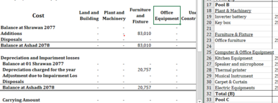
I have come across a situation where I want to add the column till there is space. Eg: Sum from B4 till there is a blank cell. Till now the value is till B6, but later it can be added to B7, B8. I cannot use an excel table in my workbook. Please refer to the attached screenshot. I need a total amount of Plant & Machinery, Furniture & Fixtures from the right sheet in my left sheet. This has to be dynamic as we keep adding machines or furniture in the coming days. What can be the best excel solution?
 

Attachments

  • Screenshot 2021-06-01 101032.png
    Screenshot 2021-06-01 101032.png
    42.9 KB · Views: 10

Excel Facts

Spell Check in Excel
Press F7 to start spell check in Excel. Be careful, by default, Excel does not check Capitalized Werds (whoops)
Welcome to the MrExcel board!

MrExcel has a tool called “XL2BB” that lets you post samples of your data that will allow us to copy/paste it to our Excel spreadsheets, so we can work with the same copy of data that you are (without having to manually type it out). Instructions on using this tool can be found here: XL2BB Add-in

Note that there is also a "Test Here” forum on this board. This is a place where you can test using this tool (or any other posting techniques that you want to test) before trying to use those tools in your actual posts.

We can't see very much in that image but it looks like there might be a total value in the right sheet in row 32. If so, how would the logic work to get a total for "Computer & Office Equipment" if there is not a blank immediately below those values?

Your profile shows both Excel 2019 & 365. Does any suggestion made need to work in both versions or would a solution in 365 only be sufficient?
 
Upvote 0
Welcome to the MrExcel board!

MrExcel has a tool called “XL2BB” that lets you post samples of your data that will allow us to copy/paste it to our Excel spreadsheets, so we can work with the same copy of data that you are (without having to manually type it out). Instructions on using this tool can be found here: XL2BB Add-in

Note that there is also a "Test Here” forum on this board. This is a place where you can test using this tool (or any other posting techniques that you want to test) before trying to use those tools in your actual posts.

We can't see very much in that image but it looks like there might be a total value in the right sheet in row 32. If so, how would the logic work to get a total for "Computer & Office Equipment" if there is not a blank immediately below those values?

Your profile shows both Excel 2019 & 365. Does any suggestion made need to work in both versions or would a solution in 365 only be sufficient?
Hi Sir,

This was overlooked because i was searching for answer in above rows. Assuming if row 32 was blank, what logic could be used to solve the issue? I would prefer the solution for both Excel 2019 & 365 because not all my collegues use 365.


Financials Format NAS for ME - V2.xlsx
ABCQRSTUVWXY
16Total (A)-CostLand and BuildingPlant & MachineryFurniture & FixtureComputer & Office EquipmentUnder ConstructionIntangiblesTotal
17Pool BBalance at Shrawan 2077-------
18Plant & MachineryAdditions-------
19Inverter battery25%1,200Disposals-------
20Key box25%1,200Balance at Ashad 2078-------
21
22Furniture & FixtureDepreciation and Impariment losses
23Office furniture25%25,000 Balance at 01 Shrawan 2077 -------
24 Depreciation charged for the year -------
25Computer & Office Equipment Adjustment due to Impairment Losses -------
26Kitchen Equipment25%5,000 Disposals ------
27Speaker and microphone25%200 Balance at Ashadh 2078 -------
28Thermal printer25%700
29Musical Instrument25%250
30Carpet & Curtain25%150
31Electric Equipments25%-
32
33Total (B)33,700
Schedule FA
Cell Formulas
RangeFormula
C16C16=C15+C10+C11
R17R17="Balance at Shrawan "&LEFT(PY_BS,4)
X17X17='Schedule FA'!T68
Y23:Y27,Y17:Y20Y17=SUM(S17:Cell_Left)
X18X18='Schedule FA'!U68
X19X19='Schedule FA'!V68
U18U18='Schedule FA'!X43
S17S17='Schedule FA'!T26
S18S18='Schedule FA'!X26
S19S19='Schedule FA'!Y26
R20R20="Balance at Ashad "&LEFT(CY_BS,4)
S20:W20S20=S17+S18-S19
X20X20='Schedule FA'!W68
R23R23="Balance at 01 Shrawan "&LEFT(PY_BS,4)
U24U24='Schedule FA'!AC43
X23X23='Schedule FA'!X68
X24X24='Schedule FA'!Y68
R27R27="Balance at Ashadh "&LEFT(CY_BS,4)
U27,X27U27=U23+U24-U25-U26
C33C33=SUM(C17:C31)
Named Ranges
NameRefers ToCells
CY_BS=Index!$I$11R20, R27
PY_BS=Index!$I$13R17, R23
 
Upvote 0
Thanks for the XL2BB data.

I'm not quite sure where you wanted the results or what column you are trying to sum (you said earlier col B but that doesn't seem right to me) but see if you can adapt this.

21 06 02.xlsm
ABCDEF
16Total (A)-
17Pool B
18Plant & MachineryPlant & Machinery2400
19Inverter battery25%1,200Furniture & Fixture25000
20Key box25%1,200Computer & Office Equipment6300
21
22Furniture & Fixture
23Office furniture25%25,000
24
25Computer & Office Equipment
26Kitchen Equipment25%5,000
27Speaker and microphone25%200
28Thermal printer25%700
29Musical Instrument25%250
30Carpet & Curtain25%150
31Electric Equipments25%-
32
33Total (B)33,700
Sum to blank
Cell Formulas
RangeFormula
F18:F20F18=SUM(INDEX(C:C,MATCH(E18,A:A,0)):INDEX(C:C,AGGREGATE(15,6,ROW(A$16:A$33)/((A$16:A$33="")*(ROW(A$16:A$33)>MATCH(E18,A:A,0))),1)))
 
Upvote 0
Solution
Wow, This is what I wanted. Thank you so much for your help.

Actually, I am trying to make a format for financial statements where when I update the trial balance financial are prepared automatically as much as possible. Are there any videos for such.
 
Upvote 0

Forum statistics

Threads
1,215,053
Messages
6,122,882
Members
449,097
Latest member
dbomb1414

We've detected that you are using an adblocker.

We have a great community of people providing Excel help here, but the hosting costs are enormous. You can help keep this site running by allowing ads on MrExcel.com.
Allow Ads at MrExcel

Which adblocker are you using?

Disable AdBlock

Follow these easy steps to disable AdBlock

1)Click on the icon in the browser’s toolbar.
2)Click on the icon in the browser’s toolbar.
2)Click on the "Pause on this site" option.
Go back

Disable AdBlock Plus

Follow these easy steps to disable AdBlock Plus

1)Click on the icon in the browser’s toolbar.
2)Click on the toggle to disable it for "mrexcel.com".
Go back

Disable uBlock Origin

Follow these easy steps to disable uBlock Origin

1)Click on the icon in the browser’s toolbar.
2)Click on the "Power" button.
3)Click on the "Refresh" button.
Go back

Disable uBlock

Follow these easy steps to disable uBlock

1)Click on the icon in the browser’s toolbar.
2)Click on the "Power" button.
3)Click on the "Refresh" button.
Go back
Back
Top