How to use the Filter function to create a single list from 3 different arrays

[Gwen0100010]

Hello,

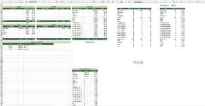
I am trying to create a single list from 3 different arrays, I am only able to get the data from 1 area at the time, And then stack the information, which is not the most efficient way to complete this spreadsheet.

Currently in U22 I have this formula =FILTER(K22:N37, K22:K37<>""). I would like this formula to include data in range A32:D37 and F32:I37 without having to add the following formula in cell U38 =FILTER(A32:D37, A32:A37<>""), O22:O37<>"") and Q42 =FILTER(F32:I37, F32:F37<>"") has I have spills issues if I modify any data in the tables

As you can see afterward the data is gathered in Table V22 who has a simple =IF(Q22<>"", Q22, "") formula do pick up the data required to create a %.

I finally use that data in K57 with this formula =SORT(FILTER(V22:X84, V22:V84<>""), 3, -1), to combine and sort the data with % and create a graph above.

I am having issues creating the graph as it takes the empty cells/values into consideration instead of only using the data with actual %.

I am sure that there is a more efficient way to create all of this and I am open to all suggestion

 

[KRice]

Are you able to post the sample worksheet using the XL2BB add-in so that the worksheet doesn't have to be re-created by anyone helping?
Also, have you considered converting the ranges mentioned (A32:D37, F32:I37, and K22:N37) into official Excel tables, perhaps named Bills, Debts, and Expenses? Then you could initially VSTACK all tables before filtering, and the "table" feature would allow the tables to expand/contract as needed without requiring any updates to the ranges.

 

[KRice]

Conceptually, this is what I tried to explain. The three source tables are named Bills, Debts, and Expenses. They are initially stacked vertically because they have the same column structure. This combined array is called "all". Then the percentages are computed based on the 3rd column (Actual relative to Total of Actuals), and that "pct" array is horizontally stacked to the "all" array...and the new 5-column array is called "rtbl"...short for revised table. Then rtbl is filtered to exclude any rows where the percentage is 0, and the resulting filtered table is sorted by column 5 (the percentages), largest to smallest. The array names are arbitrary and can be changed to your preferences. The final table displayed can also be trimmed down further to display fewer columns if desired.

MrExcel_20240415.xlsx
	A	B	C	D	E	F	G	H	I	J	K	L	M	N	O	P	Q	R	S	T
20											EXPENSES
21											NAME	BUDGET	ACTUAL	DIFF		NAME	BUDGET	ACTUAL	DIFF	PERCENTAGE
22											Groc		200			Ho	$ -	$ 300	$ -	50%
23											DO					Groc	$ -	$ 200	$ -	33%
24											Fuel					Elec	$ 100	$ 100	$ -	17%
25											Sh
26											Ho		300
27											Gi
28											Pe
29											HM
30											C1
31	BILLS					DEBTS					C2
32	NAME	BUDGET	ACTUAL	DIFF		NAME	BUDGET	ACTUAL	DIFF		C3
33	Elec	100	100			Car					C4
34	Gas										C5
35	Inter										C6
36	Water										C7
37											C8
38
Sheet2

Cell Formulas
Range	Formula
P22:T24	P22	=LET(all,VSTACK(Expenses,Bills,Debts),pct,INDEX(all,,3)/SUM(INDEX(all,,3)),rtbl,HSTACK(all,pct),SORT(FILTER(rtbl,INDEX(rtbl,,5)<>0),5,-1))
Dynamic array formulas.

 

[Gwen0100010]

Hi Krice

I have not thought of using actual table on the 3 arrays. It could make things incredibly easier. I am open to suggestion to make this much easier, as long as I get the spending breakdown results at the end and can generate the graph.

Here is a XL2BB copy of the spreadsheet. My apologies for not uploading it yesterday, I has issues with the trusted files....

Thank you so much for your help!

Budget and Finances.xlsx
	A	B	C	D	E	F	G	H	I	J	K	L	M	N	O	P	Q	R	S	T	U	V	W	X
19																						Total Expenses	$600.00
20	INCOME					SAVINGS					EXPENSES
21	INCOME NAME		EXPECTED	ACTUAL		SAVINGS NAME	BUDGET	ACTUAL	DIFF.		EXPENSES NAME	BUDGET	ACTUAL	DIFF.			Name	Budget	Actual	Diff		Name	Actual	Percentage
22			$0.00	$0.00							Groceries		$200.00	-$200.00			Groceries	0	200	-200		Groceries	200	33.33%
23			$0.00	$0.00							Dining Out		$0.00	$0.00			Dining Out	0	0	0		Dining Out	0	0.00%
24			$0.00	$0.00							Fuel		$0.00	$0.00			Fuel	0	0	0		Fuel	0	0.00%
25			$0.00	$0.00							Shopping		$0.00	$0.00			Shopping	0	0	0		Shopping	0	0.00%
26			$0.00	$0.00							Home		$300.00	-$300.00			Home	0	300	-300		Home	300	50.00%
27			$0.00	$0.00							Gifts		$0.00	$0.00			Gifts	0	0	0		Gifts	0	0.00%
28	TOTAL		$0.00	$0.00		TOTAL	$0.00	$0.00	$0.00		Pets		$0.00	$0.00			Pets	0	0	0		Pets	0	0.00%
29			$0.00								Health/Medical		$0.00	$0.00			Health/Medical	0	0	0		Health/Medical	0	0.00%
30	BILLS					DEBTS					Custom Expense 1		$0.00	$0.00			Custom Expense 1	0	0	0		Custom Expense 1	0	0.00%
31	BILLS NAME	BUDGET	ACTUAL	DIFF.		DEBT NAME	BUDGET	ACTUAL	DIFF.		Custom Expense 2		$0.00	$0.00			Custom Expense 2	0	0	0		Custom Expense 2	0	0.00%
32	Electricity	$100.00	$100.00	$0.00		Car		$0.00	$0.00		Custom Expense 3		$0.00	$0.00			Custom Expense 3	0	0	0		Custom Expense 3	0	0.00%
33	Gas		$0.00	$0.00							Custom Expense 4		$0.00	$0.00			Custom Expense 4	0	0	0		Custom Expense 4	0	0.00%
34	Internet		$0.00	$0.00							Custom Expense 5		$0.00	$0.00			Custom Expense 5	0	0	0		Custom Expense 5	0	0.00%
35	Water		$0.00	$0.00							Custom Expense 6		$0.00	$0.00			Custom Expense 6	0	0	0		Custom Expense 6	0	0.00%
36											Custom Expense 7		$0.00	$0.00			Custom Expense 7	0	0	0		Custom Expense 7	0	0.00%
37											Custom Expense 8		$0.00	$0.00			Custom Expense 8	0	0	0		Custom Expense 8	0	0.00%
38	TOTAL	$100.00	$100.00	$0.00		TOTAL	$0.00	$0.00	$0.00		TOTAL	$0.00	$500.00	-$500.00			Electricity	100	100	0		Electricity	100	16.67%
39																	Gas	0	0	0		Gas	0	0.00%
40	TRANSACTIONS TRACKER										SPENDING GRAPH						Internet	0	0	0		Internet	0	0.00%
41	DATE	AMOUNT	BUDGET NAME														Water	0	0	0		Water	0	0.00%
42	Apr-10	$200.00	Groceries														Car	0	0	0		Car	0	0.00%
43	Apr-20	$300.00	Home
44	Apr-5	$100.00	Electricity
45
46
47
48
49
50
51
52
53
54
55											SPENDING BREAKDOWN
56											BUDGET NAME	ACTUAL	PERCENTAGE
57											Home	$ 300.00	50.00%
58											Groceries	$ 200.00	33.33%
59											Electricity	$ 100.00	16.67%
60											Dining Out	$ -	0.00%
61											Fuel	$ -	0.00%
62											Shopping	$ -	0.00%
63											Gifts	$ -	0.00%
64											Pets	$ -	0.00%
65											Health/Medical	$ -	0.00%
66											Custom Expense 1	$ -	0.00%
67											Custom Expense 2	$ -	0.00%
68											Custom Expense 3	$ -	0.00%
69											Custom Expense 4	$ -	0.00%
70											Custom Expense 5	$ -	0.00%
71											Custom Expense 6	$ -	0.00%
72											Custom Expense 7	$ -	0.00%
73											Custom Expense 8	$ -	0.00%
74											Gas	$ -	0.00%
75											Internet	$ -	0.00%
76											Water	$ -	0.00%
77											Car	$ -	0.00%
78
79
80
81
82
83
84
January

Cell Formulas
Range	Formula
W19	W19	=K5
H22:H27,H32:H37	H22	=IF(ISBLANK($F22),"",SUMIF($C$42:$C$1004,$F22,$B$42:$B$1004))
I22:I27,I32:I37	I22	=IF(ISBLANK($F22),"",G22-H22)
M22:M37	M22	=IF(ISBLANK($K22),"",SUMIF($C$42:$C$1004,$K22,$B$42:$B$1004))
N22:N37	N22	=IF(ISBLANK($K22),"",L22-M22)
Q22:T37	Q22	=FILTER(K22:N37, K22:K37<>"")
V22:V48,V55:V84	V22	=IF(Q22<>"", Q22, "")
W22:W48,W55:W84	W22	=IF(Q22<>"",S22,"")
X22:X48,X55:X78	X22	=IF(V22<>"", W22/$W$19, "")
G38:I38,B38:D38,C28:D28,G28:I28	D28	=SUM(D22:D27)
C29	C29	=IF(ISBLANK(#REF!),"",SUMIF($C$42:$C$1004,#REF!,$B$42:$B$1004))
C32:C37	C32	=IF(ISBLANK($A32),"",SUMIF($C$42:$C$1004,A32,$B$42:$B$1004))
D32:D37	D32	=IF(ISBLANK($A32),"",B32-C32)
L38:N38	L38	=SUM(L21:L37)
Q38:T41	Q38	=FILTER(A32:D37, A32:A37<>"")
Q42:T42	Q42	=FILTER(F32:I37, F32:F37<>"")
U49	U49	=IF(Q49<>"", Q49, "")
X79:X84	X79	=IF(W79<>"",X79/$W$19,"")
K57:M77	K57	=SORT(FILTER(V22:X84, V22:V84<>""), 3, -1)
Dynamic array formulas.

Cells with Conditional Formatting
Cell	Condition		Cell Format	Stop If True
V21:X21	Cell	does not contain a blank value	text	NO
Q21:T21	Cell	does not contain a blank value	text	NO
K21:N21,A31,C31:D31,A38,C38:D38,K38:N38,A41:I41	Cell	does not contain a blank value	text	NO
N22:N38,D32:D38,F5,L5,I22:I29,D29,I32:I38,S36,N260:N264,N268:N298	Cell Value	<0	text	NO

 

[KRice]

Some details are missing, and depending on your workflow, what I suggested may or may not be viable. You have a Transactions Tracker. Is that manually updated, or are you drawing that information from somewhere else? Dates are associated with each transaction in the Transaction Tracker, yet no dates appear elsewhere in the Bills or Debts tables...but you do have a SUMIF formula that relies on information in the Transaction Tracker. If you log transactions for January through April, and in the Bills table, the SUMIF formula matches a Bill's Name (e.g. Electricity) to a Budget Name, do you want all Electricity transactions, or only those for a specific month or year?

How are the "names" in the Bills and Debts tables populated? Do you manually enter those or are you expecting those to be automatically generated, depending on what is found in the Transaction Tracker?

Where do the Budget numbers come from? Do you manually enter them?

 

[Gwen0100010]

This spreadsheet is for 1 month only. I have a tab for each month. I generated random dates for the transaction tacker. I thought that it would be the easiest option, I also created a dashboard that pull all data from the different tabs to it and gives an annual report.

Transaction tracker is generated manually, it is basically a copy of the bank/CC statement, and the data reported in that section adjust the data under Actual and Diff. I don't expect/need the dates to show in any other areas than in the tracker.

Budgets are manually set at the moment. I am considering having a general budget page that auto populate the monthly tabs, it really depends on the workflow after some use and tweaking.

 

[KRice]

I asked about how the Budget and Name columns were populated because a formal Table in Excel cannot use any formulas that "spill" results...and I was suggesting that you might consider converting the Bills, Debts, and Expenses ranges into formal tables. I'll add that the Transactions Tracker could also be a formal table. The example below shows this. Then the Spending Breakdown is delivered by a single spilling formula that stacks Expenses, Bills, and Debts, followed by filtering to show only those items whose "Actual" value is neither a 0 nor a blank. Then the percentages are calculated (Actual/SumActuals)...and finally, the percentages are appended to the right of the filtered compiled table and sorted based on the percentages column. Since the Spending Breakdown results are delivered by a spilling formula, you should be able to generate a Spending Graph using index references to the spilling formula cell. For example, the spilling formula is in Q22, and all results would be referenced as Q22#. If we wanted to see a pie chart showing how money was apportioned among various expenses, we would like the plot range to be dynamic, so that any number of Names appearing in the Spending Breakdown summary would appear in the Spending Graph. Ideally, we might attempt to specify INDEX(Q22#,,1) for the Names and INDEX(Q22#,,5) for the percentages directly in the data range inputs for the chart, but Excel does not accept the hash (#) spilling character for charts...so a work-around is to declare named ranges using Excel's Name Manager. For the example, I specified =INDEX(Sheet4!$Q$22#,,1) as named range "Nm" and =INDEX(Sheet4!$Q$22#,,5) as named range "Pct", and then specified Nm and Pct as the name category and percentage value to depict in the pie chart. I don't really know what you have in mind for the spending chart, but a similar strategy can be used to pull the appropriate dynamic ranges from the Spending Breakdown into the chart.

As an aside, I would strongly encourage you to avoid merged cells. Formal Excel tables do not permit them, moving data with them is difficult, and at times it may not be clear where the value appearing in a merged cell actually resided. If more space is needed (and that was the reason for merging), then consider expanding the column width, or leaving the information in the leftmost cell and then select the appropriate number of cells to the right and format them to Center Across Selection...then left justify if desired. Very similar appearance, but the data resides in a single cell and it avoids the issues with merged cells.

Book4
	A	B	C	D	E	F	G	H	I	J	K	L	M	N	O	P	Q	R	S	T	U
20	INCOME					SAVINGS					EXPENSES						SPENDING BREAKDOWN
21	INCOME NAME		EXPECTED	ACTUAL		SAVINGS NAME	BUDGET	ACTUAL	DIFF.		EXPENSES NAME	BUDGET	ACTUAL	DIFF.			Name	Budget	Actual	Diff	Percentage
22			0	0							Groceries	175	200	-25			Home	250	300	-50	42.6%
23			0	0							Dining Out		0	0			Groceries	175	200	-25	28.4%
24			0	0							Fuel		0	0			Gas	75	105	-30	14.9%
25			0	0							Shopping		0	0			Electricity	100	100	0	14.2%
26			0	0							Home	250	300	-50
27			0	0							Gifts		0	0
28	TOTAL		0	0		TOTAL	0	0	0		Pets		0	0
29			0								Health/Medical		0	0
30	BILLS					DEBTS					Custom Expense 1		0	0
31	BILLS NAME	BUDGET	ACTUAL	DIFF.		DEBT NAME	BUDGET	ACTUAL	DIFF.		Custom Expense 2		0	0
32	Electricity	100	100	0		Car		0	0		Custom Expense 3		0	0
33	Gas	75	105	-30							Custom Expense 4		0	0
34	Internet		0	0							Custom Expense 5		0	0
35	Water		0	0							Custom Expense 6		0	0
36											Custom Expense 7		0	0
37											Custom Expense 8		0	0
38	TOTAL	175	205	-30		TOTAL	0	0	0		TOTAL	425	500	-75
39
40	TRANSACTIONS TRACKER										SPENDING GRAPH
41	DATE	AMOUNT	BUDGET NAME
42	4/10/2024	200	Groceries
43	4/20/2024	300	Home
44	4/5/2024	100	Electricity
45	4/7/2024	105	Gas
Sheet4

Cell Formulas
Range	Formula
H22:H27	H22	=IF(ISBLANK($F22),"",SUMIF($C$42:$C$1005,$F22,$B$42:$B$1005))
I22:I27	I22	=IF(ISBLANK($F22),"",G22-H22)
M22:M37	M22	=IF(ISBLANK([@[EXPENSES NAME]]),"",SUMIF(Transactions[BUDGET NAME],[@[EXPENSES NAME]],Transactions[AMOUNT]))
N22:N37	N22	=IF(ISBLANK([@[EXPENSES NAME]]),"",[@BUDGET]-[@ACTUAL])
Q22:U25	Q22	=LET(all,VSTACK(Expenses,Bills,Debts),fall,FILTER(all,N(INDEX(all,,3))<>0),pct,INDEX(fall,,3)/SUM(INDEX(fall,,3)),rtbl,HSTACK(fall,pct),SORT(rtbl,5,-1))
C28:D28,G28:I28	D28	=SUM(D22:D27)
C29	C29	=IF(ISBLANK(#REF!),"",SUMIF($C$42:$C$1005,#REF!,$B$42:$B$1005))
C32:C37	C32	=IF(ISBLANK([@[BILLS NAME]]),"",SUMIF(Transactions[BUDGET NAME],[@[BILLS NAME]],Transactions[AMOUNT]))
D32:D37	D32	=IF(ISBLANK([@[BILLS NAME]]),"",[@BUDGET]-[@ACTUAL])
H32:H37	H32	=IF(ISBLANK([@[DEBT NAME]]),"",SUMIF(Transactions[BUDGET NAME],[@[DEBT NAME]],Transactions[AMOUNT]))
I32:I37	I32	=IF(ISBLANK([@[DEBT NAME]]),"",[@BUDGET]-[@ACTUAL])
B38	B38	=SUM(Bills[BUDGET])
C38	C38	=SUM(Bills[ACTUAL])
D38	D38	=SUM(Bills[DIFF.])
G38	G38	=SUM(Debts[BUDGET])
H38	H38	=SUM(Debts[ACTUAL])
I38	I38	=SUM(Debts[DIFF.])
L38	L38	=SUM(Expenses[BUDGET])
M38	M38	=SUM(Expenses[ACTUAL])
N38	N38	=SUM(Expenses[DIFF.])
Dynamic array formulas.

 

[Gwen0100010]

I did some testing and honestly it works really well. It was much simpler than what I was trying to do... I was so focused on the data gathering that I forgot to use tables..

I used this chart for the expenses and it seems to be working fine at the moment. =January!$K$42:$O$63 with some changes in the format for the labels

Would you be able to explain this formula to me? =LET(all,VSTACK(Expenses,Bills,Debts),fall,FILTER(all,N(INDEX(all,,3))<>0),pct,INDEX(fall,,3)/SUM(INDEX(fall,,3)),rtbl,HSTACK(fall,pct),SORT(rtbl,5,-1)), I am trying to wrap my head around it....

I agree, I do not like merged cells as well, I am using a format that needs to remain similar as it is being used by someone with ADHD.... I rather use center across selection.

Thank you so much for the help!!!!

Budget and Finances.xlsx
	A	B	C	D	E	F	G	H	I	J	K	L	M	N	O	P	Q	R	S	T	U	V	W	X	Y
20	INCOME					SAVINGS					EXPENSES
21	INCOME NAME	DATE	EXPECTED	ACTUAL		SAVINGS NAME	BUDGET	ACTUAL	DIFF.		EXPENSES NAME	BUDGET	ACTUAL	DIFF.
22			$0.00	$0.00							Groceries	$200.00	$200.00	$0.00
23			$0.00	$0.00							Dining Out		$0.00	$0.00
24			$0.00	$0.00							Fuel		$0.00	$0.00
25			$0.00	$0.00							Shopping		$0.00	$0.00
26			$0.00	$0.00							Home	$300.00	$300.00	$0.00
27			$0.00	$0.00							Gifts		$0.00	$0.00
28	TOTAL		$0.00	$0.00		TOTAL	$0.00	$0.00	$0.00		Pets	$150.00	$100.00	$50.00
29											Health/Medical		$0.00	$0.00
30	BILLS					DEBTS					Custom Expense 1		$0.00	$0.00
31	BILLS NAME	BUDGET	ACTUAL	DIFF.		DEBTS NAME	BUDGET	ACTUAL	DIFF.		Custom Expense 2		$0.00	$0.00
32	Electricity	$100.00	$100.00	$0.00		Car	$10.00	$10.00	$0.00		Custom Expense 3		$0.00	$0.00
33	Gas		$0.00	$0.00		Mortgage	$20.00	$30.00	-$10.00		Custom Expense 4		$0.00	$0.00
34	Internet		$0.00	$0.00							Custom Expense 5		$0.00	$0.00
35	Water		$0.00	$0.00							Custom Expense 6		$0.00	$0.00
36	Phone	$10.00	$10.00	$0.00							Custom Expense 7		$0.00	$0.00
37											Custom Expense 8		$0.00	$0.00
38	TOTAL	$110.00	$110.00	$0.00		TOTAL	$30.00	$40.00	-$10.00		TOTAL	$650.00	$600.00	$50.00
39
40	TRANSACTIONS TRACKER					SPENDING OVERVIEW					SPENDING BREAKDOWN
41	DATE	AMOUNT	BUDGET NAME	Description		BUDGET NAME	BUDGET	ACTUAL	DIFF.		BUDGET NAME	Budget	ACTUAL	Difference	PERCENTAGE
42	10-Apr-24	$200.00	Groceries			Bills	$110.00	$110.00	$0.00		Home	$ 300.00	$ 300.00	$ -	40.00%
43	20-Apr-24	$300.00	Home			Expenses	$650.00	$600.00	$50.00		Groceries	$ 200.00	$ 200.00	$ -	26.67%
44	5-Apr-24	$100.00	Electricity			Savings	$0.00	$0.00	$0.00		Pets	$ 150.00	$ 100.00	$ 50.00	13.33%
45	5-Apr-24	$10.00	Car			Debt	$30.00	$40.00	-$10.00		Electricity	$ 100.00	$ 100.00	$ -	13.33%
46	5-Apr-24	$20.00	Medical			TOTAL	$790.00	$750.00	$40.00		Mortgage	$ 20.00	$ 30.00	$ (10.00)	4.00%
47	4-Apr-24	$10.00	Phone								Phone	$ 10.00	$ 10.00	$ -	1.33%
48	5-Apr-24	$100.00	Pets								Car	$ 10.00	$ 10.00	$ -	1.33%
49	10-Apr-24	$30.00	Mortgage
50
51
52
53
54
55
56
57
58
59
January

Cell Formulas
Range	Formula
H22:H27,H32:H37	H22	=IF(ISBLANK($F22),"",SUMIF($C$42:$C$1004,$F22,$B$42:$B$1004))
I22:I27,I32:I37	I22	=IF(ISBLANK($F22),"",G22-H22)
M22:M37	M22	=IF(ISBLANK($K22),"",SUMIF($C$42:$C$1004,$K22,$B$42:$B$1004))
N22:N37	N22	=IF(ISBLANK($K22),"",L22-M22)
C28:D28,G38:I38,B38:D38,G28:I28	C28	=SUM(C22:C27)
C32:C37	C32	=IF(ISBLANK($A32),"",SUMIF($C$42:$C$1004,A32,$B$42:$B$1004))
D32:D37	D32	=IF(ISBLANK($A32),"",B32-C32)
L38:N38	L38	=SUM(L21:L37)
G42:I42	G42	=B38
G43:I43	G43	=L38
G44:I44	G44	=G28
G45:I45	G45	=G38
G46:I46	G46	=SUM(G42:G45)
K42:O48	K42	=LET(all,VSTACK(Expense,Bill,Debt),fall,FILTER(all,N(INDEX(all,,3))<>0),pct,INDEX(fall,,3)/SUM(INDEX(fall,,3)),rtbl,HSTACK(fall,pct),SORT(rtbl,5,-1))
Dynamic array formulas.

Cells with Conditional Formatting
Cell	Condition		Cell Format	Stop If True
K21:N21,A31,C31:D31,A38,C38:D38,K38:N38,A41:I41	Cell	does not contain a blank value	text	NO
N22:N37,D32:D37,F5,L5,I22:I29,D29,I32:I37,I42:I46	Cell Value	<0	text	NO

Cells with Data Validation
Cell	Allow	Criteria
C42:C59	List	=$K$42:$K$94

 

[KRice]

Sure...the formula takes advantage of some Excel 365 features that allow us to create intermediate results and assign those intermediate results to variables that we name, and then reuse later in the formula. The function that allows for this stepwise creation of intermediate results is the LET function, so consider each combination of a variable name followed by its definition as a step.

The variable names are arbitrary, so feel free to change them to something that makes sense to you, but avoid using numbers that might create a variable name that could be confused with a cell address (for example, variable names "a" and "aone" and "a_1" are fine, whereas "a1" is not). The three source tables are named Expenses, Bills, and Debts using the Table Design options.

1. In the first step, a variable called "all" is generated using the VSTACK function, which creates an array representing the vertical stacking of tables Expenses, Bills, and Debts...stacked in that order from top down. Here we assume that the source tables share common details: the same types of data in corresponding columns.
2. I noticed that these source tables sometimes have blanks (due to the formulas used in the Amount columns), and at other times we might find a 0 or some other number. Ultimately, you only want to see the entries whose Amount is a non-zero number, so it is convenient in the second step to filter out and retain only those rows in the "all" array whose Amount is a non-zero number. Also, due to the VSTACK operation, the source array columns no longer have their Name, Budget, Actual, Diff column headings, so we'll have to refer to those array columns using a different method. Typically this is where you could use the CHOOSECOLS function or the INDEX function...I chose the INDEX function, which requires us to specify the range or array and the row(s) and column(s) of interest in that range/array. The construction INDEX(all,,3) means that the "all" array will be taken (1st argument), and by leaving the 2nd argument blank, we'll get all rows of the "all" array, and by specifying 3 for the 3rd argument, we'll get the third column...which is the Actual column. Then in order to pre-condition the values in this third column, I've wrapped INDEX with the N function. The N function looks at every element in INDEX(all,,3) and delivers a 0 if the value is a blank or text, and if the value is a number, then the number will remain unchanged. This effectively converts anything that should be ignored to a 0, and we then FILTER "all" using the criteria to keep only rows associated with non-zero values in the 3rd column. Because this step trims down/filters the "all" array, I named the variable "fall"...shorted for filtered all.
3. In the third step, the variable "pct" is generated...an array of percentages based on the values in the 3rd column of "fall" (the surviving Actuals) divided by the sum of that same column. The "pct" array is a single column array of the fraction Actual/SumActuals, and each value corresponds directly to the "fall" array...so
4. In the fourth step, we horizontally stack "fall" and "pct" using the HSTACK function, which effectively appends the Percentage column to the right of the "fall" array, and this new array is called "rtbl"...I guess for revised table.
5. Finally, in the fifth step, "rtbl" is sorted using its 5th column (the percentages) from largest to smallest (the -1).

=LET(
all,  VSTACK(Expenses,Bills,Debts),
fall, FILTER(all,N(INDEX(all,,3))<>0),
pct,  INDEX(fall,,3)/SUM(INDEX(fall,,3)),
rtbl, HSTACK(fall,pct),
SORT(rtbl,5,-1)
)

 

[Gwen0100010]

That's great! I understand it much better now. and I should be able to replicate/use it in different scenario

Thank you so so so so much for all your help!