I can not use conditional formatting in Excel 2016 for Mac because the formula is too long

[renpilot]

Hello all,

I am running Excel 2016 for Mac.

I found an old thread in the forum stating that conditional formatting can only contain 256 characters. It was from2010 so I would like to verify this is still the case?

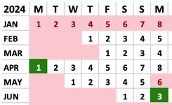
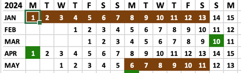
If "yes" I have a major problem in a calendar system I have created to show bookings by A,B C,D or E. I want any cell in a year to change colour if one of 45 date ranges are true. See screenshot.

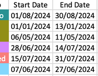
Example: A has a booking from 1/1/24 to 7/1/24 so the colour of these dates in the calendar should change colour. The same with B,C,D or E. The dates are entered as start date and end date in separate named ranges. At the bottom is an example of a formula that returns a value of true for the named ranges OURA1:OURB10 in a normal cell but can not fit in the conditional formatting formula field because it allegedly is too long.
B, C and D also has 10 possible date inputs. E has 5 possible date inputs, so all in all a lot of possible date ranges with Start Date and End Date to be checked.
The conditional formatting works with a smaller number of date entries, but when the formula gets above the 256 character length I can't write any more arguments in the conditional formatting formula field (in other words it is full).

Any help regarding how to solve this is appreciated

=OR(AND(B2>=OURA1;B2<=OURB1;B2<>"";OURA1<>"";OURB1<>"");AND(B2>=OURA2;B2<=OURB2;B2<>"";OURA2<>"";OURB2<>"");AND(B2>=OURA3;B2<=OURB3;B2<>"";OURA3<>"";OURB3<>"");AND(B2>=OURA4;B2<=OURB4;B2<>"";OURA4<>"";OURB4<>"");AND(B2>=OURA5;B2<=OURB5;B2<>"";OURA5<>"";OURB5<>"");AND(B2>=OURA6;B2<=OURB6;B2<>"";OURA6<>"";OURB6<>"");AND(B2>=OURA7;B2<=OURB7;B2<>"";OURA7<>"";OURB7<>"");AND(B2>=OURA8;B2<=OURB8;B2<>"";OURA8<>"";OURB8<>"");AND(B2>=OURA9;B2<=OURB9;B2<>"";OURA9<>"";OURB9<>"");AND(B2>=OURA10;B2<=OURB10;B2<>"";OURA10<>"";OURB10<>""))

 

[StephenCrump]

Much simpler if you put all your bookings into the one range:

	A	B	C	D	E	F	G	H	I	J	K	L	M	N	O	P	Q	R	S	T	U	V	W	X	Y	Z	AA	AB	AC	AD	AE	AF	AG	AH	AI
1
2	Booking	Start	End
3	A	1 Jan 2024	7 Jan 2024
4	B	10 Jan 2024	12 Jan 2024
5	C	13 Jan 2024	14 Jan 2024
6	D	20 Jan 2024	2 Feb 2024
7
8
9			January	1	2	3	4	5	6	7	8	9	10	11	12	13	14	15	16	17	18	19	20	21	22	23	24	25	26	27	28	29	30	31
10
Sheet1

Cells with Conditional Formatting
Cell	Condition		Cell Format	Stop If True
D9:AH9	Expression	=SUMPRODUCT(--(D9>=$B3:$B6),--(D9<=$C3:$C6))	text	NO

 

[JGordon11]

Maybe something like this?

Book1
	A	B	C	D	E	F	G	H	I	J	K	L	M	N	O	P	Q	R	S	T	U	V	W	X	Y	Z	AA	AB	AC	AD	AE	AF	AG	AH	AI
1	01	02	03	04	05	06	07	08	09	10	11	12	13	14	15	16	17	18	19	20	21	22	23	24	25	26	27	28	29	30	31		Start	End
2																																	1/3/2024	1/6/2024
3																																	1/9/2024	1/10/2024
4																																	1/15/2024	1/15/2024
5
Sheet3

Cell Formulas
Range	Formula
B1:AE1	B1	=A1+1

Cells with Conditional Formatting
Cell	Condition		Cell Format	Stop If True
A1:AE1	Expression	=SUM((A1>=$AG$2:$AG$4)*(A1<=$AH$2:$AH$4))	text	NO

 

[renpilot]

Thank you for replying.

I can see what you mean - it is simpler, but what I need is the different colour coding to give the overview. I need A, B, C, D and E to have different colours. So in case there are bookings - and also more than one from each of A, B, C, D, and E and up to a total of 45 - they show in the overview calendar as dates with different colours. I am thinking this means I have to do an ARRAY maybe as there are 12 months listed below each other?
First test if there is a booking from either A, B, C, D or E and if so assign a specific colour?
Or I could have several conditional formattings for the same range?

 

[renpilot]

I tried your second formula, but it also colours blank fields outside the calender. I have blanks as the month do not start and end on the same weekday. See attached screenshots. The green dates you see is an attempt to show holidays also if there is no booking. This particular conditional formatting works.

 

[StephenCrump]

You can include different colours like this:

	A	B	C	D	E	F	G	H	I	J	K	L	M	N	O	P	Q	R	S	T	U	V	W	X	Y	Z	AA	AB	AC	AD	AE	AF	AG	AH	AI
1
2	Booking	Start	End
3	A	1 Jan 2024	7 Jan 2024
4	B	10 Jan 2024	12 Jan 2024
5	A	13 Jan 2024	14 Jan 2024
6	C	20 Jan 2024	2 Feb 2024
7	A	5 Feb 2024	6 Feb 2024
8	B	16 Feb 2024	21 Feb 2024
9
10			January	1	2	3	4	5	6	7	8	9	10	11	12	13	14	15	16	17	18	19	20	21	22	23	24	25	26	27	28	29	30	31
11			February	1	2	3	4	5	6	7	8	9	10	11	12	13	14	15	16	17	18	19	20	21	22	23	24	25	26	27	28	29
12
Sheet1

Cells with Conditional Formatting
Cell	Condition		Cell Format	Stop If True
A3:C8	Expression	=$A3="C"	text	NO
A3:C8	Expression	=$A3="B"	text	NO
D10:AH11	Expression	=INDEX($A$3:$A$8,MATCH(1,(D10>=$B$3:$B$8)*(D10<=$C$3:$C$8),))="C"	text	NO
D10:AH11	Expression	=INDEX($A$3:$A$8,MATCH(1,(D10>=$B$3:$B$8)*(D10<=$C$3:$C$8),))="B"	text	NO
A3:C8	Expression	=$A3="A"	text	NO
D10:AH11	Expression	=INDEX($A$3:$A$8,MATCH(1,(D10>=$B$3:$B$8)*(D10<=$C$3:$C$8),))="A"	text	NO

If you post your own screenshots, please use the XL2BB - Excel Range to BBCode add-in. Then we can easily copy/paste your data and formulae.

 

[renpilot]

I have downloaded the add-on and enabled macros in Excel 2016 for Mac, but the buttons are still greyed out, so unable to upload mini sheet. See screenshot.

I got it to work with conditional formatting with this formula x 5 for each of the 5 possible entries I need:
=SUMPRODUCT(($AO$3:$AO$32="S&R")*($AP$3:$AP$32<=B2)*($AQ$3:$AQ$32>=B2))>0

However I would really like if it would be possible to have 50/50 colouring in a cell if it is booked by to parties. That means half the cell with the colour for eg S&R and the other half of the cell with the colour for eg C&B. I have tried a number of VBA codings but it does not work. Should I post this particular question somewhere else in the forum?

 

[renpilot]

I also got the two coloured format to work in a slightly different way by using conditional formatting:
=AND(SUMPRODUCT(($AO$3:$AO$32="S&R")*($AP$3:$AP$32<=B2)*($AQ$3:$AQ$32>=B2))>0;SUMPRODUCT(($AO$3:$AO$32="C&B")*($AP$3:$AP$32<=B2)*($AQ$3:$AQ$32>=B2))>0)

See screenshot

 

[StephenCrump]

I also got the two coloured format to work in a slightly different way by using conditional formatting:
=AND(SUMPRODUCT(($AO$3:$AO$32="S&R")*($AP$3:$AP$32<=B2)*($AQ$3:$AQ$32>=B2))>0;SUMPRODUCT(($AO$3:$AO$32="C&B")*($AP$3:$AP$32<=B2)*($AQ$3:$AQ$32>=B2))>0)

This might work, but you've hard-coded "S&R" and "C&B". What about the other possible permutations?

However I would really like if it would be possible to have 50/50 colouring in a cell if it is booked by to parties.

When you say two parties, do you mean something like this, where a booking turns over in the middle of the day?

	A	B	C	D	E	F	G	H	I	J	K	L	M	N	O	P	Q	R	S
1
2	Booking	Start	End
3	A	2 Jan 2024	10 Jan 2024
4	B	10 Jan 2024	13 Jan 2024
5	C	13 Jan 2024	15 Jan 2024
6
7			January	1	2	3	4	5	6	7	8	9	10	11	12	13	14	15	16
8
9
10
Sheet1

Cells with Conditional Formatting
Cell	Condition		Cell Format	Stop If True
A3:C5	Expression	=$A3="C"	text	NO
A3:C5	Expression	=$A3="B"	text	NO
A3:C5	Expression	=$A3="A"	text	NO

That's easily accommodated:

Format row 9 if Date>StartDate and Date<=EndDate
Format row 10 if Date>=StartDate and Date<EndDate

Or perhaps you want something more like this:

	A	B	C	D	E	F	G	H	I	J	K	L	M	N	O	P	Q	R	S	T	U
1
2	Booking	Unit	Start	End
3	A	1	2 Jan 2024	12 Jan 2024
4	B	2	10 Jan 2024	16 Jan 2024
5	C	1	13 Jan 2024	15 Jan 2024
6
7				January	1	2	3	4	5	6	7	8	9	10	11	12	13	14	15	16	17
8				Unit 1
9
10				Unit 2
11
12
Sheet1

Cells with Conditional Formatting
Cell	Condition		Cell Format	Stop If True
A3:D5	Expression	=$A3="C"	text	NO
A3:D5	Expression	=$A3="B"	text	NO
A3:D5	Expression	=$A3="A"	text	NO

If so, you'll just need another condition (i.e. check whether Unit = 1 or Unit =2) into your formulae.

 

[renpilot]

Thank you for your input. I have done some more research and it seems that the 50/50 colouring of 1 cell can can only be done with VBA coding.

I also had to revise my solution to only show overlaps for two people.
The way I have set it up now is actually ok and works for me with the different colours for different people and a third colour for overlapping bookings in the same line of dates which gives the overview I need

Thanks again