I want result in this formate can anyone help me

[Posting Art]

i have data in this table

Points Summary
Unit	Product Details	Staff Details	Purachase Details
Unit 1	44.28	5.00	10.00
Unit 2	-14.76	5.00	50.00
Unit 3	11.81	-2.00	-2.00
Unit 4	2.21	-1.00	-1.00
Unit 5	-8.86	0.00	5.00
Unit 6	-18.08	0.00	1.00
TOTAL	16.61	7.00	63.00

 

[maabadi]

If your Data is in Column A to D and Start from A1. Then Use This Code. You See Result At Column G to J

Sub Macro6()
Dim i As Long, j As Long, Lr As Long
   Lr = Range("A" & Rows.Count).End(xlUp).Row - 1
   Range("G4:J8").Borders.LineStyle = xlContinuous
   With Range("G4:J4")
        .Font.Bold = True
        .HorizontalAlignment = xlGeneral
        .VerticalAlignment = xlCenter
   End With
   With Range("G8:J8")
        .Font.Bold = True
        .HorizontalAlignment = xlGeneral
        .VerticalAlignment = xlCenter
   End With
    Range("G4").Value = "Description"
    Range("H4").Value = "Positive"
    Range("I4").Value = "Description"
    Range("J4").Value = "Negative"
    Range("G8").Value = "TOTAL"
    Range("H8").Formula = "=Sum(H5:H7)"
    Range("I8").Value = "TOTAL"
    Range("J8").Formula = "=Sum(J5:J7)"
    Range("H5:H8").NumberFormat = "0.00"
    Range("J5:J8").NumberFormat = "0.00"
For i = 2 To Lr
   Range("H" & (i - 2) * 10 + 2).Value = Range("A" & i).Value
   If i > 2 Then
   Range("G4:J8").Copy Range("G" & (i - 2) * 10 + 4)
   Range("G" & (i - 2) * 10 + 5 & ":J" & (i - 2) * 10 + 7).ClearContents
   End If
For j = 2 To 4
If Cells(i, j).Value >= 0 Then
Range("G" & Range("G" & (i - 2) * 10 + 8).End(xlUp).Row + 1).Value = Cells(1, j).Value
Range("H" & Range("H" & (i - 2) * 10 + 8).End(xlUp).Row + 1).Value = Cells(i, j).Value
Else
Range("I" & Range("I" & (i - 2) * 10 + 8).End(xlUp).Row + 1).Value = Cells(1, j).Value
Range("J" & Range("J" & (i - 2) * 10 + 8).End(xlUp).Row + 1).Value = Cells(i, j).Value
End If
Next j
Next i
End Sub

 

[Fluff]

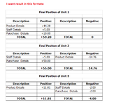
Cross-posting (posting the same question in more than one forum) is not against our rules, but the method of doing so is covered by #13 of the Forum Rules.

Be sure to follow & read the link at the end of the rule too!

Cross posted at: please help in organize data in excel sheet
If you have posted the question at more places, please provide links to those as well.

If you do cross-post in the future and also provide links, then there shouldn’t be a problem.

 

[Posting Art]

can u give me formula to do this instead of vba code?

 

[maabadi]

Not me, Maybe Others. But it is very Long & Complicated.

 

[Posting Art]

i want when i select drop down then show only selected record not all

 

[Fluff]

Now posted here please help me to organize data when i select dropdown
and also here Please help to make organized data after selection of drop drop box - OzGrid Free Excel/VBA Help Forum
@Posting Art please follow the rules in future. Thanks

 

[maabadi]

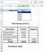
This is Macro for Create Table at Result sheet and Format it. if you have table & formatted it delete red part from code.
I suppose your sheet names are "Summary" for data and "Result" For Destination.

Sub Macro6()
Dim i As Long, j As Long, Lr As Long, Sh1 As Worksheet, Sh2 As Worksheet, M As Long, K As Long
   Set Sh1 = Sheets("Summary")
   Set Sh2 = Sheets("Result")
   Lr = Sh1.Range("A" & Rows.Count).End(xlUp).Row - 1
   M = Application.WorksheetFunction.Match(Sh2.Range("C2").Value, Sh1.Range("A1:A" & Lr), 0)
   With Sh2
   .Range("A5").Value = "Final Position of " & Sh2.Range("C2").Value
   .Range("A7:D12").Borders.LineStyle = xlContinuous
    With .Range("A7:D7")
        .Font.Bold = True
        .HorizontalAlignment = xlGeneral
        .VerticalAlignment = xlCenter
    End With
    With .Range("A12:D12")
        .Font.Bold = True
        .HorizontalAlignment = xlGeneral
        .VerticalAlignment = xlCenter
    End With
    With .Range("A5:D5")
        .Font.Bold = True
        .HorizontalAlignment = xlCenterAcrossSelection
        .VerticalAlignment = xlCenter
        .MergeCells = True
    End With
    .Range("A7").Value = "Description"
    .Range("B7").Value = "Positive"
    .Range("C7").Value = "Description"
    .Range("D7").Value = "Negative"
    .Range("A12").Value = "TOTAL"
    .Range("B12").Formula = "=Sum(B8:B11)"
    .Range("C12").Value = "TOTAL"
    .Range("D12").Formula = "=Sum(D8:D11)"
    .Range("B8:B12").NumberFormat = "0.00"
    .Range("D8:D12").NumberFormat = "0.00"
    .Range("A14").Value = "Final Result"
    .Range("C14").NumberFormat = "0.00"
    
    .Range("A8:D11").ClearContents
   
For j = 2 To 4
If Sh1.Cells(M, j).Value >= 0 Then
.Range("A" & 8 + i).Value = Sh1.Cells(1, j).Value
.Range("B" & 8 + i).Value = Sh1.Cells(M, j).Value
i = i + 1
Else
.Range("C" & 8 + K).Value = Sh1.Cells(1, j).Value
.Range("D" & 8 + K).Value = Sh1.Cells(M, j).Value
K = K + 1
End If
Next j
.Range("C14").Value = .Range("B12").Value + .Range("D12").Value
 .Columns("A:D").EntireColumn.AutoFit
End With
End Sub

if you want Worksheet change event for Result Worksheet, Right click on Result sheet name and select view Code then Paste this:

Private Sub Worksheet_Change(ByVal Target As Range)
If Intersect(Target, Range("C2")) Is Nothing Then Exit Sub
Dim i As Long, j As Long, Lr As Long, Sh1 As Worksheet, Sh2 As Worksheet, M As Long, K As Long
   Set Sh1 = Sheets("Summary")
   Set Sh2 = Sheets("Result")
   Lr = Sh1.Range("A" & Rows.Count).End(xlUp).Row - 1
   M = Application.WorksheetFunction.Match(Sh2.Range("C2").Value, Sh1.Range("A1:A" & Lr), 0)
   With Sh2
   .Range("A5").Value = "Final Position of " & Sh2.Range("C2").Value
   .Range("A7:D12").Borders.LineStyle = xlContinuous
    With .Range("A7:D7")
        .Font.Bold = True
        .HorizontalAlignment = xlGeneral
        .VerticalAlignment = xlCenter
    End With
    With .Range("A12:D12")
        .Font.Bold = True
        .HorizontalAlignment = xlGeneral
        .VerticalAlignment = xlCenter
    End With
    With .Range("A5:D5")
        .Font.Bold = True
        .HorizontalAlignment = xlCenterAcrossSelection
        .VerticalAlignment = xlCenter
        .MergeCells = True
    End With
    
    .Range("A7").Value = "Description"
    .Range("B7").Value = "Positive"
    .Range("C7").Value = "Description"
    .Range("D7").Value = "Negative"
    .Range("A12").Value = "TOTAL"
    .Range("B12").Formula = "=Sum(B8:B11)"
    .Range("C12").Value = "TOTAL"
    .Range("D12").Formula = "=Sum(D8:D11)"
    .Range("B8:B12").NumberFormat = "0.00"
    .Range("D8:D12").NumberFormat = "0.00"
    .Range("A14").Value = "Final Result"
    .Range("C14").NumberFormat = "0.00"
    
    .Range("A8:D11").ClearContents
   
For j = 2 To 4
If Sh1.Cells(M, j).Value >= 0 Then
.Range("A" & 8 + i).Value = Sh1.Cells(1, j).Value
.Range("B" & 8 + i).Value = Sh1.Cells(M, j).Value
i = i + 1
Else
.Range("C" & 8 + K).Value = Sh1.Cells(1, j).Value
.Range("D" & 8 + K).Value = Sh1.Cells(M, j).Value
K = K + 1
End If
Next j
.Range("C14").Value = .Range("B12").Value + .Range("D12").Value
.Columns("A:D").EntireColumn.AutoFit
End With
End Sub

 

[navic]

can u give me formula to do this instead of vba code?

How about,
On the Sheet "Final_Result" in the 'B8' cell formula, copy down

=IF(IFERROR(INDEX(Summary!$B$4:$E$9,MATCH($B$2,Summary!$A$4:$A$9,0),MATCH($A8,Summary!$B$3:$E$3,0)),"")>0,IFERROR(INDEX(Summary!$B$4:$E$9,MATCH($B$2,Summary!$A$4:$A$9,0),MATCH($A8,Summary!$B$3:$E$3,0)),""),"")

On the Sheet "Final_Result" in the 'C8' cell formula, copy down

=IF(IFERROR(INDEX(Summary!$B$4:$E$9,MATCH($B$2,Summary!$A$4:$A$9,0),MATCH($A8,Summary!$B$3:$E$3,0)),"")<0,IFERROR(INDEX(Summary!$B$4:$E$9,MATCH($B$2,Summary!$A$4:$A$9,0),MATCH($A8,Summary!$B$3:$E$3,0)),""),"")