Identifying data points in chart

[pholt33]

Hi,
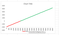
I am having trouble making a chart do what I want it to do. I have an XY scatter of dollar values, with one range for negative values so I can format the line red and another range for positive values that I can format as green. So far, so good. I have added a 3rd range of values (blue markers in pic) to identify the profit level for each 1,000 increment in revenue and the breakeven) and then I added error bars.

What I have....

Here, I started manually drawing in lines to show what I am trying to accomplish.

How can I make this happen?

Thanks!

 

[awoohaw]

please post your data in a table or xl2bb miniworkbook (preferred, link below).
This can probably be done.

 

[awoohaw]

Here is line graph:

 

[pholt33]

Let's see if this works....

Lines.xlsx
	A	B	C	D	E	F	G	H	I	J	K	L	M	N	O	P	Q	R	S	T	U	V
1			Interval	200
2
3			Revenue	Profit	Neg	Pos			Neg	Pos							X	Y
4			-	(1,852)	(1,852)	#N/A		-3.636047	(4)	#N/A			Breakeven	-	0		-	-
5			200	(1,698)	(1,698)	#N/A		-	(1,852)	#N/A			Other intervals	1,000	(1,082)		1,000	(1,082)
6			400	(1,544)	(1,544)	#N/A		150	#N/A	150				2,000	(312)		2,000	(312)
7			600	(1,390)	(1,390)	#N/A		200	(1,698)	#N/A				3,000	458		3,000	458
8			800	(1,236)	(1,236)	#N/A		400	(1,544)	#N/A				4,000	1,228		4,000	1,228
9			1,000	(1,082)	(1,082)	#N/A		600	(1,390)	#N/A				5,000	1,998		5,000	1,998
10			1,200	(928)	(928)	#N/A		800	(1,236)	#N/A				6,000	2,768		6,000	2,768
11			1,400	(774)	(774)	#N/A		1,000	(1,082)	#N/A				7,000	3,538		7,000	3,538
12			1,600	(620)	(620)	#N/A		1,200	(928)	#N/A				8,000	4,308		8,000	4,308
13			1,800	(466)	(466)	#N/A		1,400	(774)	#N/A
14			2,000	(312)	(312)	#N/A		1,600	(620)	#N/A
15			2,200	(158)	(158)	#N/A		1,800	(466)	#N/A
16			2,400	(4)	(4)	#N/A		2,000	(312)	#N/A
17			2,600	150	#N/A	150		2,200	(158)	#N/A
18			2,800	304	#N/A	304		2,400	(4)	#N/A
19			3,000	458	#N/A	458		2,600	#N/A	150
20			3,200	612	#N/A	612		2,800	#N/A	304
21			3,400	766	#N/A	766		3,000	#N/A	458
22			3,600	920	#N/A	920		3,200	#N/A	612
23			3,800	1,074	#N/A	1,074		3,400	#N/A	766
24			4,000	1,228	#N/A	1,228		3,600	#N/A	920
25			4,200	1,382	#N/A	1,382		3,800	#N/A	1,074
26			4,400	1,536	#N/A	1,536		4,000	#N/A	1,228
27			4,600	1,690	#N/A	1,690		4,200	#N/A	1,382
28			4,800	1,844	#N/A	1,844		4,400	#N/A	1,536
29			5,000	1,998	#N/A	1,998		4,600	#N/A	1,690
30			5,200	2,152	#N/A	2,152		4,800	#N/A	1,844
31			5,400	2,306	#N/A	2,306		5,000	#N/A	1,998
32			5,600	2,460	#N/A	2,460		5,200	#N/A	2,152
33			5,800	2,614	#N/A	2,614		5,400	#N/A	2,306
34			6,000	2,768	#N/A	2,768		5,600	#N/A	2,460
35			6,200	2,922	#N/A	2,922		5,800	#N/A	2,614
36			6,400	3,076	#N/A	3,076		6,000	#N/A	2,768
37			6,600	3,230	#N/A	3,230		6,200	#N/A	2,922
38			6,800	3,384	#N/A	3,384		6,400	#N/A	3,076
39			7,000	3,538	#N/A	3,538		6,600	#N/A	3,230
40			7,200	3,692	#N/A	3,692		6,800	#N/A	3,384
41			7,400	3,846	#N/A	3,846		7,000	#N/A	3,538
42			7,600	4,000	#N/A	4,000		7,200	#N/A	3,692
43			7,800	4,154	#N/A	4,154		7,400	#N/A	3,846
44			8,000	4,308	#N/A	4,308		7,600	#N/A	4,000
45		Max < 0	(4)	(4)	(4)	#N/A		7,800	#N/A	4,154
46			-	0	-	-		8,000
47		Min > 0	150	150	#N/A	150
48
Scenarios

Cell Formulas
Range	Formula
E4:E47	E4	=IF($D4<=0,$D4,NA())
F4:F47	F4	=IF($D4>=0,$D4,NA())
H4:H46	H4	=UNIQUE(SORT(C4:C47))
I4:I45	I4	=XLOOKUP($H4,$C$4:$C$47,$E$4:$E$47,,0)
J4:J45	J4	=XLOOKUP($H4,$C$4:$C$47,$F$4:$F$47,,0)
N4:O4	N4	=C46
Q4:R12	Q4	=SORT(N4:O12)
O5:O12	O5	=XLOOKUP(N5,$C$4:$C$44,$D$4:$D$44,,0)
N6:N12	N6	=N5+1000
D45	D45	=AGGREGATE(4,6,E4:E44)
C45,C47	C45	=INDIRECT("D"&MATCH(D45,D:D,0))
C46	C46	=C45 + (D46-D45) * (C47-C45) / (D47-D45)
D47	D47	=AGGREGATE(5,6,F4:F44)
Dynamic array formulas.

 

[awoohaw]

Let's see if this works....

Lines.xlsx
	A	B	C	D	E	F	G	H	I	J	K	L	M	N	O	P	Q	R	S	T	U	V
1			Interval	200
2
3			Revenue	Profit	Neg	Pos			Neg	Pos							X	Y
4			-	(1,852)	(1,852)	#N/A		-3.636047	(4)	#N/A			Breakeven	-	0		-	-
5			200	(1,698)	(1,698)	#N/A		-	(1,852)	#N/A			Other intervals	1,000	(1,082)		1,000	(1,082)
6			400	(1,544)	(1,544)	#N/A		150	#N/A	150				2,000	(312)		2,000	(312)
7			600	(1,390)	(1,390)	#N/A		200	(1,698)	#N/A				3,000	458		3,000	458
8			800	(1,236)	(1,236)	#N/A		400	(1,544)	#N/A				4,000	1,228		4,000	1,228
9			1,000	(1,082)	(1,082)	#N/A		600	(1,390)	#N/A				5,000	1,998		5,000	1,998
10			1,200	(928)	(928)	#N/A		800	(1,236)	#N/A				6,000	2,768		6,000	2,768
11			1,400	(774)	(774)	#N/A		1,000	(1,082)	#N/A				7,000	3,538		7,000	3,538
12			1,600	(620)	(620)	#N/A		1,200	(928)	#N/A				8,000	4,308		8,000	4,308
13			1,800	(466)	(466)	#N/A		1,400	(774)	#N/A
14			2,000	(312)	(312)	#N/A		1,600	(620)	#N/A
15			2,200	(158)	(158)	#N/A		1,800	(466)	#N/A
16			2,400	(4)	(4)	#N/A		2,000	(312)	#N/A
17			2,600	150	#N/A	150		2,200	(158)	#N/A
18			2,800	304	#N/A	304		2,400	(4)	#N/A
19			3,000	458	#N/A	458		2,600	#N/A	150
20			3,200	612	#N/A	612		2,800	#N/A	304
21			3,400	766	#N/A	766		3,000	#N/A	458
22			3,600	920	#N/A	920		3,200	#N/A	612
23			3,800	1,074	#N/A	1,074		3,400	#N/A	766
24			4,000	1,228	#N/A	1,228		3,600	#N/A	920
25			4,200	1,382	#N/A	1,382		3,800	#N/A	1,074
26			4,400	1,536	#N/A	1,536		4,000	#N/A	1,228
27			4,600	1,690	#N/A	1,690		4,200	#N/A	1,382
28			4,800	1,844	#N/A	1,844		4,400	#N/A	1,536
29			5,000	1,998	#N/A	1,998		4,600	#N/A	1,690
30			5,200	2,152	#N/A	2,152		4,800	#N/A	1,844
31			5,400	2,306	#N/A	2,306		5,000	#N/A	1,998
32			5,600	2,460	#N/A	2,460		5,200	#N/A	2,152
33			5,800	2,614	#N/A	2,614		5,400	#N/A	2,306
34			6,000	2,768	#N/A	2,768		5,600	#N/A	2,460
35			6,200	2,922	#N/A	2,922		5,800	#N/A	2,614
36			6,400	3,076	#N/A	3,076		6,000	#N/A	2,768
37			6,600	3,230	#N/A	3,230		6,200	#N/A	2,922
38			6,800	3,384	#N/A	3,384		6,400	#N/A	3,076
39			7,000	3,538	#N/A	3,538		6,600	#N/A	3,230
40			7,200	3,692	#N/A	3,692		6,800	#N/A	3,384
41			7,400	3,846	#N/A	3,846		7,000	#N/A	3,538
42			7,600	4,000	#N/A	4,000		7,200	#N/A	3,692
43			7,800	4,154	#N/A	4,154		7,400	#N/A	3,846
44			8,000	4,308	#N/A	4,308		7,600	#N/A	4,000
45		Max < 0	(4)	(4)	(4)	#N/A		7,800	#N/A	4,154
46			-	0	-	-		8,000
47		Min > 0	150	150	#N/A	150
48
Scenarios

Cell Formulas
Range	Formula
E4:E47	E4	=IF($D4<=0,$D4,NA())
F4:F47	F4	=IF($D4>=0,$D4,NA())
H4:H46	H4	=UNIQUE(SORT(C4:C47))
I4:I45	I4	=XLOOKUP($H4,$C$4:$C$47,$E$4:$E$47,,0)
J4:J45	J4	=XLOOKUP($H4,$C$4:$C$47,$F$4:$F$47,,0)
N4:O4	N4	=C46
Q4:R12	Q4	=SORT(N4:O12)
O5:O12	O5	=XLOOKUP(N5,$C$4:$C$44,$D$4:$D$44,,0)
N6:N12	N6	=N5+1000
D45	D45	=AGGREGATE(4,6,E4:E44)
C45,C47	C45	=INDIRECT("D"&MATCH(D45,D:D,0))
C46	C46	=C45 + (D46-D45) * (C47-C45) / (D47-D45)
D47	D47	=AGGREGATE(5,6,F4:F44)
Dynamic array formulas.

which is the section you want charted?

 

[pholt33]

H:J are the red and green lines. Q:R are the blue dots with error bars.

 

[awoohaw]

H:J are the red and green lines. Q:R are the blue dots with error bars.

im confused. where did error bars and blue dots come from? I thought you were plotting revenue vs profit.
I took profit and split it up in to loss/gain, plotted against revenue.

But, my problem is I can't get x axis to be numerical. It looks numerical but the spacing is not. Strange.

 

[awoohaw]

I've adjusted your data to have both values at switch over show up on the POS/NEG lines to ensure line connectivity.

mr excel questions 34.xlsm
	H	I	J	K
1
2
3	Rent	Cashflow	Neg	Pos
4	0	-1851.636047	-1851.636047	#N/A
5	200	-1697.636047	-1697.636047	#N/A
6	400	-1543.636047	-1543.636047	#N/A
7	600	-1389.636047	-1389.636047	#N/A
8	800	-1235.636047	-1235.636047	#N/A
9	1000	-1081.636047	-1081.636047	#N/A
10	1200	-927.636047	-927.636047	#N/A
11	1400	-773.636047	-773.636047	#N/A
12	1600	-619.636047	-619.636047	#N/A
13	1800	-465.636047	-465.636047	#N/A
14	2000	-311.636047	-311.636047	#N/A
15	2200	-157.636047	-157.636047	#N/A
16	2400	-3.636046986	-3.636046986	-3.636046986
17	2600	150.363953	150.363953	150.363953
18	2800	304.363953	#N/A	304.363953
19	3000	458.363953	#N/A	458.363953
20	3200	612.363953	#N/A	612.363953
21	3400	766.363953	#N/A	766.363953
22	3600	920.363953	#N/A	920.363953
23	3800	1074.363953	#N/A	1074.363953
24	4000	1228.363953	#N/A	1228.363953
25	4200	1382.363953	#N/A	1382.363953
26	4400	1536.363953	#N/A	1536.363953
27	4600	1690.363953	#N/A	1690.363953
28	4800	1844.363953	#N/A	1844.363953
29	5000	1998.363953	#N/A	1998.363953
30	5200	2152.363953	#N/A	2152.363953
31	5400	2306.363953	#N/A	2306.363953
32	5600	2460.363953	#N/A	2460.363953
33	5800	2614.363953	#N/A	2614.363953
34	6000	2768.363953	#N/A	2768.363953
35	6200	2922.363953	#N/A	2922.363953
36	6400	3076.363953	#N/A	3076.363953
37	6600	3230.363953	#N/A	3230.363953
38	6800	3384.363953	#N/A	3384.363953
39	7000	3538.363953	#N/A	3538.363953
40	7200	3692.363953	#N/A	3692.363953
41	7400	3846.363953	#N/A	3846.363953
42	7600	4000.363953	#N/A	4000.363953
43	7800	4154.363953	#N/A	4154.363953
44	8000	4308.363953	#N/A	4308.363953
pholt33_2

Cell Formulas
Range	Formula
J4:J44	J4	=IF($D4<0,$D4,IF(AND(D4>=0,N(D3)<=0),D4,NA()))
K4:K44	K4	=IF(OR($D4>0,AND($D4<0,$D5>=0)),$D4,NA())

 

[pholt33]

im confused. where did error bars and blue dots come from? I thought you were plotting revenue vs profit.
I too profit and split it up in to loss/gain, plotted against revenue.

But, my problem is I can't get x axis to be numerical. Strange.

The blue dots are from Q4:R12, which is a subset of the full data but only for 1,000 increments plus the breakeven amount. Those plot on top of the red and green lines. I did that so it would (theoretically) be easier to do the lines I want.

 

[awoohaw]

The blue dots are from Q4:R12, which is a subset of the full data but only for 1,000 increments plus the breakeven amount. Those plot on top of the red and green lines. I did that so it would (theoretically) be easier to do the lines I want.

View attachment 90891

then do the same for those as with neg/pos... put a value of NA() in the cells that are not in the number intervals you want.

for the dots, you can add markers and change their size in any of the series options. I don't think you need to create a new series just for that..

but I was also looking into "drop" and "High Low" Lines but those don't seem to work as I think you want.