If and AND function

[DeekMan]

Good afternoon,
I have created a formula using IF & AND functions, it seems rather long winded, is there a more elagant way of writing this formula.

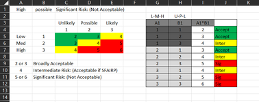
The job is to put an answer in C1 (it will be a column in the final sheet) based on the two answers in A1 and A2, the formula does work, and I did try adding the OR function, but unfortunatly I managed to get myself lost.

=IF(AND(A1="Low",B1="Unlikely"),"Broardly Acceptable Risk",IF(AND(A1="Low",B1="Possible"),"Broardly Acceptable Risk",IF(AND(A1="Med",B1="Unlikely"),"Broardly Acceptable Risk",IF(AND(A1="Low",B1="Likely"),"Intermediate Risk: (Acceptable if SFAIRP)",IF(AND(A1="Med",B1="Possible"),"Intermediate Risk: (Acceptable if SFAIRP)",IF(AND(A1="High",B1="Unlikely"),"Intermediate Risk: (Acceptable if SFAIRP)",IF(AND(A1="Med",B1="Likely"),"Significant Risk: (Not Acceptable)",IF(AND(A1="High",B1="Possible"),"Significant Risk: (Not Acceptable)",IF(AND(A1="High",B1="Likely"),"Significant Risk: (Not Acceptable)")))))))))

Many thanks in advance.

 

[etaf]

a few ways to do that
but as you have mentioned OR
try

=IF(OR(AND(A1="Low",B1="Unlikely"),AND(A1="Low",B1="Possible"),AND(A1="Med",B1="Unlikely")),"Broardly Acceptable Risk",
IF(OR(AND(A1="Low",B1="Likely"),AND(A1="Med",B1="Possible"),AND(A1="High",B1="Unlikely")),"Intermediate Risk: (Acceptable if SFAIRP)",
IF(OR(AND(A1="Med",B1="Likely"),AND(A1="High",B1="Possible"),AND(A1="High",B1="Likely")),"Significant Risk: (Not Acceptable)","if all false")))

Grouping the common TRUE outputs together

you may want a FALSE condition , as i have shown , otherwise you just get FALSE in the cell if none met

Not sure how to apply to the image, as i'm not sure what results you are looking for where , doesnt seem to match with the IF() formula you added

do you want to lookup - whatever is put into a1 and b1 - then the table you have could be used , if you just put the words into a column and the result - i'll try an mock something up and post a new reply

may be able to use the TABLE to lookup values - rather than the Nested IF() - which will mean any changes are much easier

depending on version of excel - maybe other ways

what version do you have - would be worth updating your profile

Note: Images are difficult to see , and also requires that I input all the data myself, which means I may make an error, which is very time consuming, and from my point of view less likely to get a response, if a complicated spreadsheet. Plus we cannot see any of the formulas used.

Therefore -

A SMALL sample spreadsheet, around 10-20 rows, would help a lot here, with all sensitive data removed, and expected results mocked up and manually entered, with a few notes of explanation.

This will possibly enable a quicker and more accurate solution for you.

MrExcel has a tool called “XL2BB” that lets you post samples of your data and will allow us to copy/paste your sample data into our Excel spreadsheets, saving a lot of time.

XL2BB - Excel Range to BBCode

Excel 'mini-sheet' in messages - XL2BB Although experts prefer to read your description and question instead of working in your actual file to solve your problem, there are times that it is difficult to explain an issue without providing actual...

www.mrexcel.com

You can also test to see if it works ok, in the "Test Here" forum.

Test Here

Use this forum to test your signature, learn bbcode, smilies, XL2BB, etc. Threads in this forum are automatically deleted after no replies for seven (7) days

www.mrexcel.com

OR if you cannot get XL2BB to work, or have restrictions on your PC

then put the sample spreadsheet onto a share

I only tend to goto OneDrive, Dropbox or google docs , as I'm never certain of other random share sites and possible virus.
Please make sure you have a representative data sample and also that the data has been desensitised, remember this site is open to anyone with internet access to see - so any sensitive / personal data should be removed

Make sure you set any share or google to share to everyone

 

[etaf]

in C1 on my example is the IF
=IF(OR(AND(A1="Low",B1="Unlikely"),AND(A1="Low",B1="Possible"),AND(A1="Med",B1="Unlikely")),"Broardly Acceptable Risk",
IF(OR(AND(A1="Low",B1="Likely"),AND(A1="Med",B1="Possible"),AND(A1="High",B1="Unlikely")),"Intermediate Risk: (Acceptable if SFAIRP)",
IF(OR(AND(A1="Med",B1="Likely"),AND(A1="High",B1="Possible"),AND(A1="High",B1="Likely")),"Significant Risk: (Not Acceptable)","if all false")))

in D1 in my example is the lookup - with an added column to the table
=INDEX($I$4:$I$12,MATCH(A1&B1,$G$4:$G$12&$H$4:$H$12,0))

Book14
	A	B	C	D	E	F	G	H	I	J
1	high	likely	Significant Risk: (Not Acceptable)	Significant Risk: (Not Acceptable)
2			if all false	#N/A
3	low	unlikely	Broardly Acceptable Risk	Broardly Acceptable Risk
4	low	possible	Broardly Acceptable Risk	Broardly Acceptable Risk			low	unlikely	Broardly Acceptable Risk
5	low	likely	Intermediate Risk: (Acceptable if SFAIRP)	Intermediate Risk: (Acceptable if SFAIRP)			low	possible	Broardly Acceptable Risk
6	med	unlikely	Broardly Acceptable Risk	Broardly Acceptable Risk			low	likely	Intermediate Risk: (Acceptable if SFAIRP)
7	med	possible	Intermediate Risk: (Acceptable if SFAIRP)	Intermediate Risk: (Acceptable if SFAIRP)			med	unlikely	Broardly Acceptable Risk
8	med	likely	Significant Risk: (Not Acceptable)	Significant Risk: (Not Acceptable)			med	possible	Intermediate Risk: (Acceptable if SFAIRP)
9	high	unlikely	Intermediate Risk: (Acceptable if SFAIRP)	Intermediate Risk: (Acceptable if SFAIRP)			med	likely	Significant Risk: (Not Acceptable)
10	high	possible	Significant Risk: (Not Acceptable)	Significant Risk: (Not Acceptable)			high	unlikely	Intermediate Risk: (Acceptable if SFAIRP)
11	high	likely	Significant Risk: (Not Acceptable)	Significant Risk: (Not Acceptable)			high	possible	Significant Risk: (Not Acceptable)
12							high	likely	Significant Risk: (Not Acceptable)
13
Sheet1

Cell Formulas
Range	Formula
C1:C11	C1	=IF(OR(AND(A1="Low",B1="Unlikely"),AND(A1="Low",B1="Possible"),AND(A1="Med",B1="Unlikely")),"Broardly Acceptable Risk", IF(OR(AND(A1="Low",B1="Likely"),AND(A1="Med",B1="Possible"),AND(A1="High",B1="Unlikely")),"Intermediate Risk: (Acceptable if SFAIRP)", IF(OR(AND(A1="Med",B1="Likely"),AND(A1="High",B1="Possible"),AND(A1="High",B1="Likely")),"Significant Risk: (Not Acceptable)","if all false")))
D1:D11	D1	=INDEX($I$4:$I$12,MATCH(A1&B1,$G$4:$G$12&$H$4:$H$12,0))

 

[Peter_SSs]

I suggest that you update your Account details (or click your user name at the top right of the forum) so helpers always know what Excel version(s) & platform(s) you are using as the best solution often varies by version. (Don’t forget to scroll down & ‘Save’)

I have abbreviated some of the result texts but you can fill them out if this does what you want.

23 05 21.xlsm
	A	B	C
1	High	Possible	Significant
2	High	Unlikely	Intermediate
3	High	Likely	Significant
4	Low	Possible	Broadly Acceptable
5	Low	Unlikely	Broadly Acceptable
6	Low	Likely	Intermediate
7	Medium	Possible	Intermediate
8	Medium	Unlikely	Broadly Acceptable
9	Medium	Likely	Significant
DeekMan

Cell Formulas
Range	Formula
C1:C9	C1	=LOOKUP(MATCH(A1,{"Low","Medium","High"},0)+MATCH(B1,{"Unlikely","Possible","Likely"},0),{2,4,5},{"Broadly Acceptable","Intermediate","Significant"})

 

[DeekMan]

a few ways to do that
but as you have mentioned OR
try

=IF(OR(AND(A1="Low",B1="Unlikely"),AND(A1="Low",B1="Possible"),AND(A1="Med",B1="Unlikely")),"Broardly Acceptable Risk",
IF(OR(AND(A1="Low",B1="Likely"),AND(A1="Med",B1="Possible"),AND(A1="High",B1="Unlikely")),"Intermediate Risk: (Acceptable if SFAIRP)",
IF(OR(AND(A1="Med",B1="Likely"),AND(A1="High",B1="Possible"),AND(A1="High",B1="Likely")),"Significant Risk: (Not Acceptable)","if all false")))

Grouping the common TRUE outputs together

you may want a FALSE condition , as i have shown , otherwise you just get FALSE in the cell if none met

Not sure how to apply to the image, as i'm not sure what results you are looking for where , doesnt seem to match with the IF() formula you added

do you want to lookup - whatever is put into a1 and b1 - then the table you have could be used , if you just put the words into a column and the result - i'll try an mock something up and post a new reply

may be able to use the TABLE to lookup values - rather than the Nested IF() - which will mean any changes are much easier

depending on version of excel - maybe other ways

what version do you have - would be worth updating your profile

Note: Images are difficult to see , and also requires that I input all the data myself, which means I may make an error, which is very time consuming, and from my point of view less likely to get a response, if a complicated spreadsheet. Plus we cannot see any of the formulas used.

Therefore -

A SMALL sample spreadsheet, around 10-20 rows, would help a lot here, with all sensitive data removed, and expected results mocked up and manually entered, with a few notes of explanation.

This will possibly enable a quicker and more accurate solution for you.

MrExcel has a tool called “XL2BB” that lets you post samples of your data and will allow us to copy/paste your sample data into our Excel spreadsheets, saving a lot of time.

XL2BB - Excel Range to BBCode

Excel 'mini-sheet' in messages - XL2BB Although experts prefer to read your description and question instead of working in your actual file to solve your problem, there are times that it is difficult to explain an issue without providing actual...

www.mrexcel.com

You can also test to see if it works ok, in the "Test Here" forum.

Test Here

Use this forum to test your signature, learn bbcode, smilies, XL2BB, etc. Threads in this forum are automatically deleted after no replies for seven (7) days

www.mrexcel.com

OR if you cannot get XL2BB to work, or have restrictions on your PC

then put the sample spreadsheet onto a share

I only tend to goto OneDrive, Dropbox or google docs , as I'm never certain of other random share sites and possible virus.
Please make sure you have a representative data sample and also that the data has been desensitised, remember this site is open to anyone with internet access to see - so any sensitive / personal data should be removed

Make sure you set any share or google to share to everyone

Many thanks for your solution. I can see now where I was going wrong with the OR & AND, I had =IF(OR(AND(A1xxxxxxxxxxx) but didnt have the extra AND between the next (A1xxxxxxxxxx) I have tried your solution and it works fine. Thnak You.

 

[DeekMan]

in C1 on my example is the IF
=IF(OR(AND(A1="Low",B1="Unlikely"),AND(A1="Low",B1="Possible"),AND(A1="Med",B1="Unlikely")),"Broardly Acceptable Risk",
IF(OR(AND(A1="Low",B1="Likely"),AND(A1="Med",B1="Possible"),AND(A1="High",B1="Unlikely")),"Intermediate Risk: (Acceptable if SFAIRP)",
IF(OR(AND(A1="Med",B1="Likely"),AND(A1="High",B1="Possible"),AND(A1="High",B1="Likely")),"Significant Risk: (Not Acceptable)","if all false")))

in D1 in my example is the lookup - with an added column to the table
=INDEX($I$4:$I$12,MATCH(A1&B1,$G$4:$G$12&$H$4:$H$12,0))

Book14
	A	B	C	D	E	F	G	H	I	J
1	high	likely	Significant Risk: (Not Acceptable)	Significant Risk: (Not Acceptable)
2			if all false	#N/A
3	low	unlikely	Broardly Acceptable Risk	Broardly Acceptable Risk
4	low	possible	Broardly Acceptable Risk	Broardly Acceptable Risk			low	unlikely	Broardly Acceptable Risk
5	low	likely	Intermediate Risk: (Acceptable if SFAIRP)	Intermediate Risk: (Acceptable if SFAIRP)			low	possible	Broardly Acceptable Risk
6	med	unlikely	Broardly Acceptable Risk	Broardly Acceptable Risk			low	likely	Intermediate Risk: (Acceptable if SFAIRP)
7	med	possible	Intermediate Risk: (Acceptable if SFAIRP)	Intermediate Risk: (Acceptable if SFAIRP)			med	unlikely	Broardly Acceptable Risk
8	med	likely	Significant Risk: (Not Acceptable)	Significant Risk: (Not Acceptable)			med	possible	Intermediate Risk: (Acceptable if SFAIRP)
9	high	unlikely	Intermediate Risk: (Acceptable if SFAIRP)	Intermediate Risk: (Acceptable if SFAIRP)			med	likely	Significant Risk: (Not Acceptable)
10	high	possible	Significant Risk: (Not Acceptable)	Significant Risk: (Not Acceptable)			high	unlikely	Intermediate Risk: (Acceptable if SFAIRP)
11	high	likely	Significant Risk: (Not Acceptable)	Significant Risk: (Not Acceptable)			high	possible	Significant Risk: (Not Acceptable)
12							high	likely	Significant Risk: (Not Acceptable)
13
Sheet1

Cell Formulas
Range	Formula
C1:C11	C1	=IF(OR(AND(A1="Low",B1="Unlikely"),AND(A1="Low",B1="Possible"),AND(A1="Med",B1="Unlikely")),"Broardly Acceptable Risk", IF(OR(AND(A1="Low",B1="Likely"),AND(A1="Med",B1="Possible"),AND(A1="High",B1="Unlikely")),"Intermediate Risk: (Acceptable if SFAIRP)", IF(OR(AND(A1="Med",B1="Likely"),AND(A1="High",B1="Possible"),AND(A1="High",B1="Likely")),"Significant Risk: (Not Acceptable)","if all false")))
D1:D11	D1	=INDEX($I$4:$I$12,MATCH(A1&B1,$G$4:$G$12&$H$4:$H$12,0))

Good Afternoon, Thank you for your solution - I hadn't thought about a lookup table. Thank you.

 

[DeekMan]

I suggest that you update your Account details (or click your user name at the top right of the forum) so helpers always know what Excel version(s) & platform(s) you are using as the best solution often varies by version. (Don’t forget to scroll down & ‘Save’)

I have abbreviated some of the result texts but you can fill them out if this does what you want.

23 05 21.xlsm
	A	B	C
1	High	Possible	Significant
2	High	Unlikely	Intermediate
3	High	Likely	Significant
4	Low	Possible	Broadly Acceptable
5	Low	Unlikely	Broadly Acceptable
6	Low	Likely	Intermediate
7	Medium	Possible	Intermediate
8	Medium	Unlikely	Broadly Acceptable
9	Medium	Likely	Significant
DeekMan

Cell Formulas
Range	Formula
C1:C9	C1	=LOOKUP(MATCH(A1,{"Low","Medium","High"},0)+MATCH(B1,{"Unlikely","Possible","Likely"},0),{2,4,5},{"Broadly Acceptable","Intermediate","Significant"})

I have updated my profile, as you suggested.
This is looks to be a very simple formula, but it does every thing that I need. I have never used "match" before. I am assuming that the lookup element is is using the data within the { } , I am not sure what the },0) zero is for, likewise I dont know what the ,{2,4,5}, is for. but I do know it works.
Many thanks.

 

[Peter_SSs]

I have updated my profile, as you suggested.

Thanks for doing that.

To explain the formula look at this example from my earlier post.

23 05 21.xlsm
	A	B	C
4	Low	Possible	Broadly Acceptable
DeekMan

Cell Formulas
Range	Formula
C4	C4	=LOOKUP(MATCH(A4,{"Low","Medium","High"},0)+MATCH(B4,{"Unlikely","Possible","Likely"},0),{2,4,5},{"Broadly Acceptable","Intermediate","Significant"})

=LOOKUP(MATCH(A4,{"Low","Medium","High"},0)+MATCH(B4,{"Unlikely","Possible","Likely"},0),{2,4,5},{"Broadly Acceptable","Intermediate","Significant"})
=LOOKUP(MATCH("Low",{"Low","Medium","High"},0)+MATCH("Possible",{"Unlikely","Possible","Likely"},0),{2,4,5},{"Broadly Acceptable","Intermediate","Significant"})
The MATCH is looking for the underlined word within the { } and returns the position it is found. The ,0 at the end of the MATCH tells the MATCH to look for an exact match.
So the blue match returns 1 since "Low" is the first word in the blue curly brackets and the red match returns 2 since "Possible" is the second word in the red curly brackets.
The formula then becomes
=LOOKUP(1+2,{2,4,5},{"Broadly Acceptable","Intermediate","Significant"})
=LOOKUP(3,{2,4,5},{"Broadly Acceptable","Intermediate","Significant"})

LOOKUP looks for 3 in the first curly brackets (Which must be in ascending order). It cannot find a 3 in this case so it returns the next lowest number that is in the brackets, which is 2.
2 is in the first position in the first brackets so LOOKUP returns the value from the first position in the second brackets: "Broadly Acceptable"

 

[DeekMan]

Thanks for doing that.

To explain the formula look at this example from my earlier post.

23 05 21.xlsm
	A	B	C
4	Low	Possible	Broadly Acceptable
DeekMan

Cell Formulas
Range	Formula
C4	C4	=LOOKUP(MATCH(A4,{"Low","Medium","High"},0)+MATCH(B4,{"Unlikely","Possible","Likely"},0),{2,4,5},{"Broadly Acceptable","Intermediate","Significant"})

=LOOKUP(MATCH(A4,{"Low","Medium","High"},0)+MATCH(B4,{"Unlikely","Possible","Likely"},0),{2,4,5},{"Broadly Acceptable","Intermediate","Significant"})
=LOOKUP(MATCH("Low",{"Low","Medium","High"},0)+MATCH("Possible",{"Unlikely","Possible","Likely"},0),{2,4,5},{"Broadly Acceptable","Intermediate","Significant"})
The MATCH is looking for the underlined word within the { } and returns the position it is found. The ,0 at the end of the MATCH tells the MATCH to look for an exact match.
So the blue match returns 1 since "Low" is the first word in the blue curly brackets and the red match returns 2 since "Possible" is the second word in the red curly brackets.
The formula then becomes
=LOOKUP(1+2,{2,4,5},{"Broadly Acceptable","Intermediate","Significant"})
=LOOKUP(3,{2,4,5},{"Broadly Acceptable","Intermediate","Significant"})

LOOKUP looks for 3 in the first curly brackets (Which must be in ascending order). It cannot find a 3 in this case so it returns the next lowest number that is in the brackets, which is 2.
2 is in the first position in the first brackets so LOOKUP returns the value from the first position in the second brackets: "Broadly Acceptable"

Peter,

Many thanks for the explanation. This is very clever.
Sorry for the delay in responding, its been a busy week.

Deek.

 

[Peter_SSs]

Cheers.