If cell does not contain specific text, then return a that missing text

[Aharris90]

Hello,
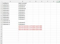
I am hoping someone can help. I am trying to run a formula that will search a column for text and if that text does not match text within another column to then return the missing text to the bottom of the column the text is missing from.

So lets say Column A has 100 records and Column B has 75 records, I would like row 76 in column B to return the first missing text from Column A.

I hope that makes sense.

Thanks

 

[RobP]

Hi

not quite sure to understand exactly, but would you not just use "=a1" in cell B1, and then copy the formula down the page to the empty cells ?

From your description above, you are suggesting that your desired goal is to have column B = to Column A ?

Is that correct ?

maybe some examples of actual (or dummy) data might help ?

thanks
Rob

 

[Aharris90]

Hi Rob,

Thanks for your reply. I have attached a screenshot of some dummy Data. Column "Query Data" is pulled from our database and is a list of customers that have actually ordered with us in the year. Column "Sales Forecast" is a list of the customer sales said they would take an order from.

What we are trying to do is track the accuracy of the sales forecasts. So we are having the file lookup where the names match in the two columns and pull throught the acutal order value vs the forecasted value which is easy.

The part we are now trying to solve is that there could be a customer in Column "Query Data" that is not in Column "Sales Forecast" as we perhaps never knew about that customer when we did the forecast so rather than having to spot the ones that are missing in Column "Sales Forecast" compared to "Query Data" manually we would like it to enter the text to the bottom of the "Sales Forecast" Column. AS you see in that data Customer 12 we have received an order for but we did not expect it as the sales team did not forecast it. We would therefore like a formula that will add the text "Customer 12" or whatever the name of the missing customers are in the column "Sales Forecast". Then as we run the query each week as more add in for the formula to keep adding them from Column A to the bottom of Column B where I have placed the red Text.

It seems simplier in this limited data size to spot but the real data has 600 customers and the order is not the same in each column. Does that help?

 

[kvsrinivasamurthy]

In B12 then copy down

=IFERROR(INDEX($A$2:$A$13,Aggregata(15,6,ROW($A$2:$A$13)/(COUNTIF($B$2:$B$10,$A$2:$A$13)=0),ROWS($B$12:$B12))-ROW($A$1)),"")

 

[RobP]

Hi,

yes, thats a lot more clear, thankyou.

The downside is that I don't know of a "formula" that can handle that. A formula can act on data, but will only return a result in a specific cell if you understand me well. So for each customer thats missing, you would need an appropriate formula in the same number of cells. But of course you dont know how many are missing, so you dont know how many formulas you need to add to your sheet. I dont think its possible for a formula to act on multiple items either (eg. more than 1 missing customer).

So, it would mean some VBA code in a Macro to do the work. (which is possible). Are you familiar with VBA code at all, where it gets stored, how its run etc.? Do you have access to the "Developer" tab ?
thanks
Rob

 

[RobP]

ah ok, looks like Srini is much more knowledgeable than me ! (as are most!)
Rob

 

[Aharris90]

Thanks Rob. I have used VBA a really small amount and do have access to the Developer tab but am quite new to VBA to be honest. I have tried the suggestion above by Kvsrinivasamurhty but that did not return all missing values.

 

[Aharris90]

@kvsrinivasamurthy if I understand your suggest correct it is working based on the gap in the dummy data set in column B. They may have been a little misleading as the data will be in consistent lists without gaps. I showed it like this to help the explanation.

​

 

[Fluff]

How about

Fluff.xlsm
	A	B
1	County	County
2	West Midlands	Wiltshire
3	Northumberland	County Durham
4	Devon	Staffordshire
5	Cheshire	Somerset
6	Cornwall	North Yorkshire
7	Gloucestershire	West Yorkshire
8	Kent	East Riding of Yorkshire
9	Merseyside	Greater Manchester
10	East Riding of Yorkshire	Merseyside
11	Norfolk	Tyne and Wear
12	Nottinghamshire	Essex
13	Staffordshire	Cheshire
14	Hertfordshire	Greater London
15	Lancashire	Derbyshire
16	West Yorkshire	Nottinghamshire
17	Lincolnshire
18	Wiltshire
19	County Durham	West Midlands
20	Somerset	Northumberland
21	North Yorkshire	Devon
22	Greater Manchester	Cornwall
23		Gloucestershire
24		Kent
25		Norfolk
26		Hertfordshire
27		Lancashire
28		Lincolnshire
29
Main

Cell Formulas
Range	Formula
B19:B28	B19	=FILTER(A2:A22,ISNA(MATCH(A2:A22,B2:B16,0)))
Dynamic array formulas.

 

[Aharris90]

That is it! Thank you Fluff