If formula and Indirect formula

[Ev1lZer0]

I am trying to get color bands on similar dates while having alternating colors on the rest of the table. I started by using an IF formula and had "=IF(A1=A2,B1,NOT(B1))" I also had come conditional formatting involved.
If you need more information, I am using the process shown on the website. "Colour Bands in Excel Table Based on Dates – Contextures Blog"

It works really well, except for when I insert or delete rows. Which will happen frequently.

When I add rows, I get an inconsistent formula error; when I delete rows I get a #REF error. These errors always start BELOW the inserted row.

---

To resolve this, I tried using an INDIRECT formula with the IF formula and ended up with this. =IF((ADDRESS(ROW()-1,COLUMN()-1))=(ADDRESS(ROW(),COLUMN()-1)),B9,NOT(B9)) it does not work. It is now alternating my true false statement incorrectly. in addition, the [value if false] and [value if true] statement is still referencing the cell above which ends up breaking the formula in the same way I stated earlier.
When I add rows, I get an inconsistent formula error; when I delete rows I get a #REF error. These errors always start BELOW the inserted row.

---

lastly, I tried changing the formula to "=IF((ADDRESS(ROW()-1,COLUMN()-1))=(ADDRESS(ROW(),COLUMN()-1)),(ADDRESS(ROW()-1,COLUMN())),NOT(ADDRESS(ROW()-1,COLUMN())))" My hope was to resolve the #REF error and Inconsistent formula error and address the issue where this formula seems to not correctly label true false.

--

I'm pulling out my hair and desperately need help

The end goal... to alternate color bands based on similar dates like the image below. The true and false should be alternated while similar dates should be grouped together and alternated.

And to state again, the solution needs to work when adding or deleting cells - mine in the past have not.

 

[cmowla]

Hi.

This can be done with (at most) 2 helper columns + 2 conditional formatting rules.

• You can hide the two helper columns.
• IF you append/include these two helper columns in the Excel Table itself, then you don't need to carry these formulas down.
• This conditional formatting will work, even if rows are filtered/hidden.
• Note: Under the column named "Cells with Conditional Formatting" (specifically, under Cell) in the image below, that's the range that the conditional formatting formula "Applies to". With the Excel Table, when you add a new row, it will automatically change the conditional formatting "Applies to" range. (You just have to set it up just ONCE.)
• But it appears that if you delete a row, you will have to re-carrydown the formulas in the helper columns. (So if there is indeed no way arround that, either you get someone to write a VBA script for you to unhide the 2 helper columns and recarry down the formula or manually do it after you have deleted all rows that you want to.)

Book1.xlsx
	A	B	C	D
1	Date of Trial	TRUE	Date of Trial (Helper)	TRUE (Helper)
2	9/6/2022	FALSE	1	2
3	9/6/2022	TRUE	2	3
4	9/12/2022	TRUE	1	4
5	9/12/2022	TRUE	2	5
6	9/12/2022	TRUE	3	6
7	9/12/2022	TRUE	4	7
8	9/12/2022	TRUE	5	8
9	9/12/2022	TRUE	6	9
10	9/12/2022	TRUE	7	10
11	9/12/2022	TRUE	8	11
12	9/12/2022	TRUE	9	12
13	9/12/2022	TRUE	10	13
14	9/12/2022	TRUE	11	14
15	9/12/2022	TRUE	12	15
16	9/12/2022	TRUE	13	16
17	9/12/2022	TRUE	14	17
18	9/19/2022	FALSE	1	18
19	9/19/2022	FALSE	2	19
20	9/20/2022	TRUE	1	20
21	9/21/2022	FALSE	1	21
22	9/22/2022	TRUE	1	22
23	9/23/2022	FALSE	1	23
24	9/26/2022	TRUE	1	24
25	9/26/2022	TRUE	2	25
26	9/26/2022	TRUE	3	26
27	9/26/2022	TRUE	4	27
Sheet2 (2)

Cell Formulas
Range	Formula
C2:C27	C2	=IF(A2=A1,COUNTIF($A$2:A2,A2),1*IF(SUBTOTAL(103,A1)>0,1,0))
D2:D27	D2	=IF(SUBTOTAL(103,A2)>0,1,0)*ROW()

Cells with Conditional Formatting
Cell	Condition		Cell Format	Stop If True
B2:B27	Expression	=MOD(D2,2)=0	text	NO
A2:A27	Expression	=MOD(COUNTIF($C$2:C2,1),2)=0	text	NO

 

[cmowla]

While I'm at it, here is VBA code that will create a button that, when you click on it, it will carry down the formula (in the Date of Trial Helper column) for you. But note that when you click on this button, you cannot undo any action you did before clicking on it! Therefore, if you decide to use it, here is the code and instructions.

1. See my signature for instructions on how to enable VBA macros/code if you want to use it (and have never used macros/VBA before).
   
   
2. After you do that, press Alt+F11 to bring up the code window.
   
   
3. In the left margin, you will see a list of sheets like this (if not, press Ctrl + R to bring it up).
   
   
   
   
   
4. Right click on any of those sheets and insert a new module:
   
   
   
   
   
5. Copy all of the code in the code block below inside of it.

Option Explicit

Sub Test__Create_Button()
Call Create_Button("G1:G2", ActiveSheet.Name, "Test__Update_Table")
End Sub

Sub Test__Update_Table()
Call Update_Table("Table3", "Date of Trial", "Date of Trial (Helper)")
End Sub

Sub Create_Button(cellAddress As String, sheetName As String, macroNameToRun As String)

Sheets(sheetName).Buttons.Delete

With Sheets(sheetName).Range(cellAddress)
    Dim btn As Button
    Set btn = Sheets(sheetName).Buttons.Add(.Left, .Top, .Width, .Height)
End With

With btn
    .Font.Size = 12
    .Font.Bold = False
    .Font.Name = "Calibri"
    .OnAction = macroNameToRun
    .Caption = "Fix"
    .Name = sheetName & "_Fix Button_" & cellAddress
End With

End Sub
Sub Update_Table(tableName$, dateOfTrialColumnName$, helperColumnName$)

On Error GoTo Let_User_Know
With Range(tableName)
    Dim headerRow&
    headerRow = .Rows(1).Row - 1

    Dim helperColumnNumber%
    helperColumnNumber = Trim(Evaluate("MATCH(" & Chr(34) & helperColumnName & Chr(34) & "," & headerRow & ":" & headerRow & ",0)"))

    'If at least 1 row was deleted from the table (there is at least one cell with #REF! error in the helper column),
    If Evaluate("SUM(IFERROR(" & tableName & "[" & helperColumnName & "]*0,1))") > 0 Then

        Dim firstRow&
        firstRow = headerRow + 1

        Dim numberOfRowsInTable&
        numberOfRowsInTable = .Rows.Count

        Dim dateOfTrialColumnNumber%
        dateOfTrialColumnNumber = Trim(Evaluate("MATCH(" & Chr(34) & dateOfTrialColumnName & Chr(34) & "," & headerRow & ":" & headerRow & ",0)"))

        Dim colLetter$
        colLetter = Split(Cells(1, dateOfTrialColumnNumber).Address, "$")(1)

        Dim helperColumnRange As Range
        Set helperColumnRange = Range(Cells(firstRow, helperColumnNumber), Cells(firstRow + numberOfRowsInTable - 1, helperColumnNumber))
        helperColumnRange.Formula2 = _
            "=IF(" & colLetter & firstRow & "=" & colLetter & headerRow & ",COUNTIF($" & colLetter & "$" & firstRow & ":" & _
            colLetter & firstRow & "," & colLetter & firstRow & "),1*IF(SUBTOTAL(103," & colLetter & headerRow & ")>0,1,0))"
    End If

End With

Exit Sub
Let_User_Know:
MsgBox "You need to name the table, the trial date heading, and trial date helper column heading what you have them named (verbatim) in this sheet's code module.", vbCritical, "Filling down formula failed."

End Sub

Notes (and final steps):

• There are 4 Subs in the code block above. You don't need to modify the 3rd and 4th (long) subs.
  
  
• In the first sub, you need to change the "G1:G2" to whatever cell(s) you want the button to be placed on. (Placing it on multiple cells allows to make the button larger.)
  
  
• In the second sub, you need to change the table name from Table3 to whatever the name of your table is in your sheet (keep the quotes).
  
  
  
  
  
• In the second sub, also be sure that the heading of Date of Trial is whatever you named your "Date of Trial" column in your table (verbatim . . . no Alt+Enter vertical spaces or extra spaces to wrap text, etc.).
  
  
• (But of course, type Date of Trial (Helper). This will ensure that this button will work.)
  
  
• Once all of that is finished, click anywhere on the middle line in the first sub and then click on the green play button to create the button. (If at any time you wish to delete the button, right click on it and select Cut.)
  
  

 

[cmowla]

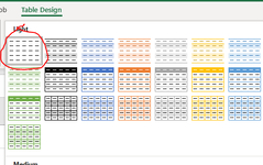
And this reminds me, in order for formatting of Excel Tables to not "conflict" with the conditional formatting, you need to select this (blank) formatting option for the table if it isn't already:

Final Note:
The conditional formatting for column B (TRUE/FALSE) will only work if the first row of data is on an even row number. So if you want to offset the table vertically down from the top, it needs to be that the first data row starts on row 4, 6, etc. (if not where you have it currently at row 2).

 

[Fluff]

Another option without any helper columns

Fluff.xlsm
	A
1	Date of Trial
2	09/06/2022
3	09/06/2022
4	09/12/2022
5	09/12/2022
6	09/12/2022
7	09/12/2022
8	09/12/2022
9	09/12/2022
10	09/12/2022
11	09/12/2022
12	09/12/2022
13	09/12/2022
14	09/12/2022
15	09/12/2022
16	09/12/2022
17	09/12/2022
18	19/09/2022
19	19/09/2022
20	20/09/2022
21	21/09/2022
22	22/09/2022
23	23/09/2022
24	26/09/2022
25	26/09/2022
26	26/09/2022
27	26/09/2022
Main

Cells with Conditional Formatting
Cell	Condition		Cell Format	Stop If True
A2:A27	Expression	=MOD(SUMPRODUCT(--($A$2:$A2<>$A$1:$A1)),2)=0	text	NO

 

[cmowla]

@Fluff , but your solution doesn't hold if rows in the table are filtered. I assume that this is a desired/expected feature (since the table in the OP has filters). Can you modify it so that it does accompany that constraint? (And also make a CF for Column B?)

 

[Fluff]

The OP made no mention of filtering the data & the formula I suggested replicates what the OP is doing with the helper column.

 

[cmowla]

Okay, I guess we will have to wait and see if keeping the CF when the table is filtered is important.

 

[Ev1lZer0]

I am going to play with both of these options.

At first glance, it seems that @Fluff's solution may work, but I will have to experiment with the filters to see if keeping the CF is actually important.

To be honest, I hope it's not, since this seems like a much simpler way of 'fixing things' than @cmowla's way. At the end of the day, I am just creating the spreadsheet, it will be others that utilize it on a regular basis. Either direction I go, I am super appreciative of the help and will report back my findings.

Thank you!

 

[Fluff]

If you filter the data the the CF may not work as you want, but it will be the same as the way you were using.