If/ifs formula help

[Sophiepope]

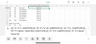
I have the below data.
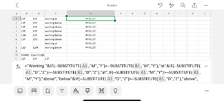
I have the current formula in which works for all the data apart from row 3 - returns working above but in fact is working below.

=ifs(a1=b1,”working at”,a1>b1,”working above”,a1<b1,”working below”)

Does anyone know how I can amend the formula. I cannot ask it to ignore all instances of the + symbol as that would create incorrect data in other cells e.g row 5.

A B C
4+ 4+ working at
4+ 3 Working above
4+ 6 Working above
4 4+ working below
4+ 4 Working above

 

[Peter_SSs]

I suggest that you update your Account details (or click your user name at the top right of the forum) so helpers always know what Excel version(s) & platform(s) you are using as the best solution often varies by version. (Don’t forget to scroll down & ‘Save’)

 

[Peter_SSs]

In relation to my above comment, depending on which Excel version you are using, here are a couple of options that I think do what you want.

24 04 05.xlsm
	A	B	C	D
1	4+	4+	Working at	Working at
2	4+	3	Working above	Working above
3	4+	6	Working below	Working below
4	4	4+	Working below	Working below
5	4+	4	Working above	Working above
at above below

Cell Formulas
Range	Formula
C1:C5	C1	=LET(a,--SUBSTITUTE(A1,"+",".1"),b,--SUBSTITUTE(B1,"+",".1"),"Working "&IF(a=b,"at",IF(a>b,"above","below")))
D1:D5	D1	="Working "&IF(--SUBSTITUTE(A1,"+",".1")=--SUBSTITUTE(B1,"+",".1"),"at",IF(--SUBSTITUTE(A1,"+",".1")>--SUBSTITUTE(B1,"+",".1"),"above","below"))

 

[Sophiepope]

The formula in column D worked perfectly. Thank you for your help.
Could you assist which how to add IFERROR in also. I would like it to be a blank box if it’s an error if possible.
Thank you in advance

 

[Peter_SSs]

Thanks for updating your version details.

Could you assist which how to add IFERROR in also. I would like it to be a blank box if it’s an error if possible.

This should do it but it might be better we knew what sort of data you had that caused the error in the first place.

=IFERROR("Working "&IF(--SUBSTITUTE(A2,"+",".1")=--SUBSTITUTE(B2,"+",".1"),"at",IF(--SUBSTITUTE(A2,"+",".1")>--SUBSTITUTE(B2,"+",".1"),"above","below")),"")

 

[Sophiepope]

That sorted it. The error was being cause by empty cells.
Thank you very much for your help.

 

[Peter_SSs]

OK, cheers.

 

[Sophiepope]

apologies, following on from the above thread I am having a similar issue but this time with text. I am using the below formula:

=IFERROR("Working "&IF(--SUBSTITUTE(A1,"M","Y")=--SUBSTITUTE(B1,"M","Y"),"at"&IF(--SUBSTITUTE(A1,"D","Z")=--SUBSTITUTE(B1,"D","Z"),"at",IF(--SUBSTITUTE(A1,"M","Y")>--SUBSTITUTE(B1,"M","Y"),"above","below"&IF(--SUBSTITUTE(A1,"D","Z")>--SUBSTITUTE(B1,"D","Z"),"above","below")))),"")

But just getting blank returns.
I have results such as 1D and 1P. A regular formula returns ‘working below’ but should be showing as ‘working above’
I can only think that the letter P is higher in the alphabet than D, therefor I have tried to change it to a Z so it would be higher than the P but it still pulls through blank. It does the same with an M which should be also showing as higher so attempted to change this to a Y.

I hope this makes sense and any help is much appreciated.

 

[Peter_SSs]

I hope this makes sense

It doesn't to me. You have given a formula that does not work for you, no variety of sample data, no explanation of what letters are used, what they mean etc. Could we have 5-10 rows of sample data with the expected results manually filled in and explain why those are the expected results? Please use XL2BB (If you have trouble with XL2BB review the "XL2BB Icons greyed out" link in the 'Known XL2BB issues' section near the top of theXL2BB Instructions page linked above.) so that we can easily see copy/paste the sample data and know what rows/columns it is is.

 

[Sophiepope]

Hello,
Thank you for your response. Unfortunately at the time of asking I was using a work desktop and am now not in the office for a couple of day - I tried to get mini sheet on my IPhone but this doesn’t seem to be an option - I have added photo’s incase this would help. If not I’m happy to try and get a mini sheet sorted when I return and send it over.
If the below images do help please see below:

Picture 1 - shows a standard formula which does pull through a valid response but I have some issues where is does not pull correctly. The numbers and letters are detailed in picture 1 from lowest to highest going down and then across.
Picture 2 - shows a more complex formula whereby I ask it to substitute the letters ‘D’ for a ‘Z’ and an ‘M’ for a ‘Y’. This I need it to return a ‘working above’ response when column a=L2D and column b=L2P.

Please let me know if this doesn’t help - as I can completely understand having a mini sheet to physically work on is easier.

Thank you for your help