If less than, divide by...

[Bedford]

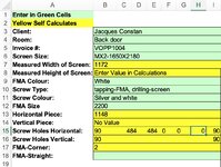
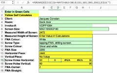
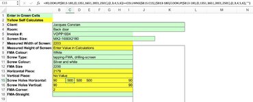
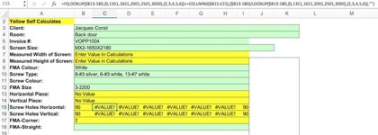
Attempting a calculation. A cell (B13) results in a whole number based on a formula. That resulting whole number is dynamic, example; 2179. Then 2179-180=1999, 180 is static. The result 1999, needs to be divided by 2 if <1350, divided by 3 if > 1351 but < 1650, divided by 4 if > 1651 but < 2000, divided by 5 if > 2001 but < 2500, divided by 6 if > 2501 but < 3000.
I'm hoping this can be done in a formula, and that someone can assist.
Thank you in advance.

 

[Bedford]

Perhaps it would be better if @Bedford could show some examples with actual values and expected results in order to eliminate any more potential confusion from convoluted descriptions.

I hope this makes sense?

 

[jasonb75]

The description in your post makes sense now that I've seen the screen capture.
Enter this into C15 and fill down.

=IF(ROWS($C$15:$C15)<=MATCH(B13-180,{0,1351,1651,2001,2501}),$C$13,"")

 

[Bedford]

The description in your post makes sense now that I've seen the screen capture.
Enter this into C15 and fill down.

=IF(ROWS($C$15:$C15)<=MATCH(B13-180,{0,1351,1651,2001,2501}),$C$13,"")

I entered the formula in C15, but the result is zero. Is it meant to be an array?

 

[jtakw]

I hope this makes sense?

The description in your post makes sense now that I've seen the screen capture.

Actually, it does not, in your Post #7, you wanted to use C15:C19, but the screenshot you show in Post #11 appears that you're using D15:H15.
And Now, your post #13 appears your may have "Merged" cells...

This works in C15 dragged across to G15, without merged cells:

Book3.xlsx
	B	C	D	E	F	G
13	1148
14
15		484
Sheet833

Cell Formulas
Range	Formula
C15:G15	C15	=IF(LOOKUP($B13-180,{0,1351,1651,2001,2501},{2,3,4,5,6})>=COLUMNS($B15:C15),($B13-180)/LOOKUP($B13-180,{0,1351,1651,2001,2501},{2,3,4,5,6}),"")

If this works for you, we'll see if we can shorten the formula a bit.

 

[Bedford]

Actually, it does not, in your Post #7, you wanted to use C15:C19, but the screenshot you show in Post #11 appears that you're using D15:H15.
And Now, your post #13 appears your may have "Merged" cells...

This works in C15 dragged across to G15, without merged cells:

Book3.xlsx
	B	C	D	E	F	G
13	1148
14
15		484
Sheet833

Cell Formulas
Range	Formula
C15:G15	C15	=IF(LOOKUP($B13-180,{0,1351,1651,2001,2501},{2,3,4,5,6})>=COLUMNS($B15:C15),($B13-180)/LOOKUP($B13-180,{0,1351,1651,2001,2501},{2,3,4,5,6}),"")

If this works for you, we'll see if we can shorten the formula a bit.

So true, added columns and it copied merged cells, sorry for the mess I've been working at this one for seems too long. That said, your formula works! I dragged across from C15 to H15, it added results in C15:E15, since it's calculating dividing B13 by 4, I'm hoping it will return results only in C15:F15, if dividing by 5, it should return results C15:G15, and likewise if dividing by only 2 results to C15:C16.

 

[jtakw]

I've tested my formula using different values in B13 and it's working according to your description, you should test with various possible scenarios for your data.
Let us know if the formula needs modification.

 

[Bedford]

So true, added columns and it copied merged cells, sorry for the mess I've been working at this one for seems too long. That said, your formula works! I dragged across from C15 to H15, it added results in C15:E15, since it's calculating dividing B13 by 4, I'm hoping it will return results only in C15:F15, if dividing by 5, it should return results C15:G15, and likewise if dividing by only 2 results to C15:C16.

Actually, it does not, in your Post #7, you wanted to use C15:C19, but the screenshot you show in Post #11 appears that you're using D15:H15.
And Now, your post #13 appears your may have "Merged" cells...

This works in C15 dragged across to G15, without merged cells:

Book3.xlsx
	B	C	D	E	F	G
13	1148
14
15		484
Sheet833

Cell Formulas
Range	Formula
C15:G15	C15	=IF(LOOKUP($B13-180,{0,1351,1651,2001,2501},{2,3,4,5,6})>=COLUMNS($B15:C15),($B13-180)/LOOKUP($B13-180,{0,1351,1651,2001,2501},{2,3,4,5,6}),"")

If this works for you, we'll see if we can shorten the formula a bit.

Sorry, my mistake, it works in every way, all good, EUREKA, thank you very much!

 

[jtakw]

You're welcome, thanks for the feedback, glad we figured it out.

 

[Bedford]

You're welcome, thanks for the feedback, glad we figured it out.

Such a wonderful forum. Great thanks again.

 

[Bedford]

You're welcome, thanks for the feedback, glad we figured it out.

I'm sorry to rehash, this formula you provided works great, one thing if I could ask. When the source cell; B13 contains "No Value" due to B7 containing literally no value from its source, B7 is referencing; =IF(Calculations!C10<>"",Calculations!C10,IF(Calculations!C15<>"",Calculations!C15,IF(Calculations!C20<>"",Calculations!C20,IF(Calculations!C26<>"",Calculations!C26,IF(Calculations!C31<>"",Calculations!C31,IF(Calculations!C36<>"",Calculations!C36,"Enter Value In Calculations"))))))
Therefore C15 is returning an error #VALUE! as it's attempting to calculate the text result; "Enter Value In Calculations". Is there a work around for correcting the #VALUE! error in C15 when B13 is not returning a numeric value?