If this Cell Range contains True in each field, Highlight this different range in the same colour, No

[billsfree]

Hi.

New to Excel and was wondering if someone might be kind enough to lend me a hand

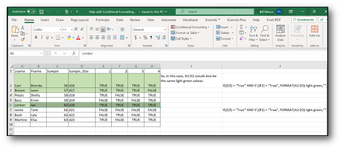
I have an Excel Worksheet with 8 columns:
The first range is D1:D4 (All Text Values)

The range adjacent is D5:D8 (All Boolean values)

Conditional Formatting formula: If(D5 AND D6 AND D7 AND D8) = True, Highlight the 8 fields in light green, otherwise do not do anything...

If((E2:H2) = "True", FORMAT(A2:D2) light green,""))

Sorry.. this is probably a stupid question but I have been working on this and trying to figure it out but just cannot get the range A2:D2 to also be light green if the range D1:D4 all equal true.
Another idea I had is maybe it is easier to refenece the row ? For example, if the 4 columns are true then highlight the row to light green, otherwise leave the row as it is...

Thanks for taking the time to read my Post and I hope you have an awesome Thursday !!!

Oblio

 

[etaf]

you can have whatever colour you want - just how its going to be selected and setup -
may need 2 formulas
one as we have
Select G3:H1000
=AND($G3="DVNY", $H3="DVNY")
which will be green and white
and then
Select A3:F1000
=AND($E3="Yes",$F3="Yes", $G3="DVNY", $H3="DVNY")

confrm-etaf-V5.xlsx
	A	B	C	D	E	F	G	H
1
2
3					yes	yes	yes	yes
4
5					yes	no	yes	yes
6							DVNY
7					yes	yes		DVNY
8					Yes	yes	DVNY	DVNY
9							DVNY	DVNY
10
11
12
13
14
15
Sheet1

Cells with Conditional Formatting
Cell	Condition		Cell Format	Stop If True
A3:F1000	Expression	=AND($E3="Yes", $F3="Yes", $G3="DVNY", $H3="DVNY")	text	NO
G3:H1000	Expression	=COUNTIF($G3:$H3,"DVNY")=2	text	YES
E3:H1000	Expression	=E3="yes"	text	NO
A3:H1000	Expression	=COUNTIF($E3:$H3,"yes")=4	text	NO

Dropbox - File Deleted - Simplify your life

www.dropbox.com

 

[billsfree]

you can have whatever colour you want - just how its going to be selected and setup -
may need 2 formulas
one as we have
Select G3:H1000
=AND($G3="DVNY", $H3="DVNY")
which will be green and white
and then
Select A3:F1000
=AND($E3="Yes",$F3="Yes", $G3="DVNY", $H3="DVNY")

confrm-etaf-V5.xlsx
	A	B	C	D	E	F	G	H
1
2
3					yes	yes	yes	yes
4
5					yes	no	yes	yes
6							DVNY
7					yes	yes		DVNY
8					Yes	yes	DVNY	DVNY
9							DVNY	DVNY
10
11
12
13
14
15
Sheet1

Cells with Conditional Formatting
Cell	Condition		Cell Format	Stop If True
A3:F1000	Expression	=AND($E3="Yes", $F3="Yes", $G3="DVNY", $H3="DVNY")	text	NO
G3:H1000	Expression	=COUNTIF($G3:$H3,"DVNY")=2	text	YES
E3:H1000	Expression	=E3="yes"	text	NO
A3:H1000	Expression	=COUNTIF($E3:$H3,"yes")=4	text	NO

Dropbox - File Deleted - Simplify your life

www.dropbox.com

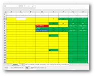
Okay, that formula makes sense, now and everything is working perfectly other than I am trying to force UPPER(A3:H1000) but I am getting a circular reference warning.
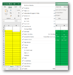
I have tried even just doing one random cell and it does not force to upper. I right clicked on the error tab on the bottom left to try and add Uppercase from that menu, but nothing changed...

Do I need to do something special because of the conditional formatting in order to force Uppercase ? What about Propercase (First Letter Capital and the rest lower case Both Firstname and Lastname).

Thanks, Wayne, very much.

How's the weather today in England ?

 

[etaf]

Weather is great , down on the coast

you cannot do that on the cell its self, upper would change the text to another cell - so in J3 for example - UPPER(E3) would put uppecase in

you could add Data Validation , so they can only enter uppercase or proper case into the cell

I have added 2 data validation rules
one for column A - so only PROPER can be entered - you also get a message up to do that
and column E to H - for uppercase only

is that something that would work -

confrm-etaf-V7.xlsx
	A	B	C	D	E	F	G	H
3					YES	YES	YES	YES
4
5					YES	NO	YES	YES
6							DVNY
7					YES	YES		DVNY
8					YES	YES	DVNY	DVNY
9							DVNY	DVNY
10
11
12
13					YES
14
15
16
17
18
19
20
21
22
23
24
25
26
27
28
29
30
31
32
33
Sheet1

Cells with Conditional Formatting
Cell	Condition		Cell Format	Stop If True
A3:F1000	Expression	=AND($E3="Yes", $F3="Yes", $G3="DVNY", $H3="DVNY")	text	NO
G3:H1000	Expression	=COUNTIF($G3:$H3,"DVNY")=2	text	YES
E3:H1000	Expression	=E3="yes"	text	NO
A3:H1000	Expression	=COUNTIF($E3:$H3,"yes")=4	text	NO

Cells with Data Validation
Cell	Allow	Criteria
A3:A33	Custom	=PROPER(A3)
E3:H33	Custom	=UPPER(E3)

I have selected A3:A1000
then gone to data validation
custom
entered
=PROPER(A3)
then put an input message and an error message

then selected E3:H1000
then gone to data validation
custom
entered
=UPPER(E3)
then put an input message and an error message

Dropbox - File Deleted - Simplify your life

www.dropbox.com

 

[etaf]

Further to last post - it could be done with a macro VBA - but i dont provide solutions using VBA , so if you want to have a button to click and rthen all the entries are replaced with the format you want - you could post a new question in the forum - and see what answers you get
it maybe possible with Power Query - but i dont do that either , as on a MAC its only recently been available

you should also update your profile to show what version of Excel you have - 2007/2010/2013/2016/2019/2021 or subscription version 365
and the platform - Windows 7/8/10/11 or OSX (Mac)

 

[billsfree]

Further to last post - it could be done with a macro VBA - but i dont provide solutions using VBA , so if you want to have a button to click and rthen all the entries are replaced with the format you want - you could post a new question in the forum - and see what answers you get
it maybe possible with Power Query - but i dont do that either , as on a MAC its only recently been available

you should also update your profile to show what version of Excel you have - 2007/2010/2013/2016/2019/2021 or subscription version 365
and the platform - Windows 7/8/10/11 or OSX (Mac)

I will for certain right away !

Very interesting about validation help text and errors... I will tuck that away in my new basket of tricks thanks to you !

Macros are something I have never tried... for now, I think we will leave the Caps required off and error messages... I thought it was me not entering UPPER() properly, so thanks for showing me that, too !

Just tried moving existing data to the new Conditional Format Spreadsheet. Most is correcr, However, I am getting some errors where blank cells are... so I will need to check the proper rules... There was no mention of Yellow cells in the Conditional formatting so I am thinking we just colour the whole spreadsheet Yellow and let the conditional format change cells that require it ? Or should I be more concerned ?

Well, I am glad to hear you have had some GOOD weather... my gosh, the crazy things happening lately

I am into Geneology and took the DNA test... 99 percent UK, lol so interesting... one day I hope to do a tour. Berwick Upon Tweed, The Cleethorpes, Cotswolds, London, Lancashire, Wooten-Under-Edge and on and on... then there's an irish line a french line a german line... I guess were a European "Mutt" lol.

Good night, Wayne, and again SO MANY THANKS for your amazing help and knowledge... you have the patience of JOB, sir !!!

Have a good evening !

 

[etaf]

There was no mention of Yellow cells in the Conditional formatting so I am thinking we just colour the whole spreadsheet Yellow and let the conditional format change cells that require it ? Or should I be more concerned ?

post 21

you could just format the whole area yellow to begin with

so yes just colour the whole area A3:H1000 YELLOW

Most is correcr, However, I am getting some errors where blank cells are..

let me know the details and i should be able to help , unless its the yellow issue which answered