If this Cell Range contains True in each field, Highlight this different range in the same colour, No

[billsfree]

Hi.

New to Excel and was wondering if someone might be kind enough to lend me a hand

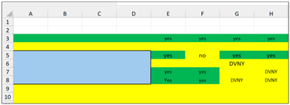
I have an Excel Worksheet with 8 columns:
The first range is D1:D4 (All Text Values)

The range adjacent is D5:D8 (All Boolean values)

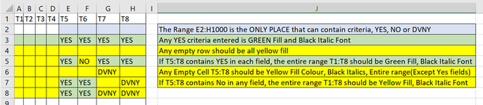
Conditional Formatting formula: If(D5 AND D6 AND D7 AND D8) = True, Highlight the 8 fields in light green, otherwise do not do anything...

If((E2:H2) = "True", FORMAT(A2:D2) light green,""))

Sorry.. this is probably a stupid question but I have been working on this and trying to figure it out but just cannot get the range A2:D2 to also be light green if the range D1:D4 all equal true.
Another idea I had is maybe it is easier to refenece the row ? For example, if the 4 columns are true then highlight the row to light green, otherwise leave the row as it is...

Thanks for taking the time to read my Post and I hope you have an awesome Thursday !!!

Oblio

 

[billsfree]

I really cannot thank you enough !!! Just trying to modify it to Yes or No so I will need to go over it again to make sure I understand it... Again SO many thanks !!!

 

[billsfree]

ok,
changing what to yes/no - if we can help let us know

Good Grief, I thought it woulld be no issue to just trade "TRUE" to "YES", and the only other change my boss wants is for any "NO" to be format filled Yellow, or if all 4 columns have nothing entered, this should have all 4 cells yellow. When I changed TRUE to YES in the formulas, I got the #Name Error.

Afraid I am all mixed up :/

So, can I start asking where do I put the:

=COUNTIF($E2:$H2,TRUE)=4

in I3 ? and then if it equals 4 Add conditional formatting for that field, value is Equal to 4 would make the whole line green.

BUT I also need each Individual YES to be Green, as well...Do I also conditionally Format Each Cell=Yes is green in case there is a NO field... so the whole line would not all be green due to the NO Entered.

How does each cell return a 1 if True. It does not seem to count YES instead as all I get is a zero when I try subsituting YES for TRUE...

 

[etaf]

i may not answer now till Saturday - going out now - UK Timezone

as yes is text it needs to be "yes" in inverted commas


but you will need 3 rules and 3 selections - i think

first
=countif($E2:$H2,"yes")=4
for A2 to H26 or whatever the full range is

for 2007, 2010 , 2013 , 2016 , 2019 or 365 Subscription excel version
Conditional Formatting

Highlight applicable range >>
A2:H100 - Change, reduce or extend the rows to meet your data range of rows

Home Tab >> Styles >> Conditional Formatting
New Rule >> Use a formula to determine which cells to format
Edit the Rule Description: Format values where this formula is true:
=countif($E2:$H2,"yes")=4

Format [Number, Font, Border, Fill] Green
choose the format you would like to apply when the condition is true
OK >> OK

that will do each line if all 4 are YES
next
select E2:H100 or whatever the rows are
then
Highlight applicable range >>
E2:H100 - Change, reduce or extend the rows to meet your data range of rows

Home Tab >> Styles >> Conditional Formatting
New Rule >> Use a formula to determine which cells to format
Edit the Rule Description: Format values where this formula is true:
=E2="yes"

Format [Number, Font, Border, Fill] GREEN
choose the format you would like to apply when the condition is true
OK >> OK
next rule
next
select E2:H100 or whatever the rows are
then
Highlight applicable range >>
E2:H100 - Change, reduce or extend the rows to meet your data range of rows

Home Tab >> Styles >> Conditional Formatting
New Rule >> Use a formula to determine which cells to format
Edit the Rule Description: Format values where this formula is true:
=E2="NO"

Format [Number, Font, Border, Fill] Yellow
choose the format you would like to apply when the condition is true
OK >> OK

Book8
	A	B	C	D	E	F	G	H
1
2					yes	yes	yes	yes
3							no
4
5					no	yes	no	no
6					yes	yes	yes	yes
7					no	yes	no	yes
Sheet1

Cells with Conditional Formatting
Cell	Condition		Cell Format	Stop If True
E2:H7	Expression	=E2="no"	text	NO
E2:H7	Expression	=E2="yes"	text	NO
A2:H7	Expression	=COUNTIF($E2:$H2,"yes")=4	text	NO

I have also added the file onto dropbox - only be there for a few days -

Dropbox - File Deleted - Simplify your life

www.dropbox.com

 

[billsfree]

i may not answer now till Saturday - going out now - UK Timezone

as yes is text it needs to be "yes" in inverted commas


but you will need 3 rules and 3 selections - i think

first
=countif($E2:$H2,"yes")=4
for A2 to H26 or whatever the full range is

for 2007, 2010 , 2013 , 2016 , 2019 or 365 Subscription excel version
Conditional Formatting

Highlight applicable range >>
A2:H100 - Change, reduce or extend the rows to meet your data range of rows

Home Tab >> Styles >> Conditional Formatting
New Rule >> Use a formula to determine which cells to format
Edit the Rule Description: Format values where this formula is true:
=countif($E2:$H2,"yes")=4

Format [Number, Font, Border, Fill] Green
choose the format you would like to apply when the condition is true
OK >> OK

that will do each line if all 4 are YES
next
select E2:H100 or whatever the rows are
then
Highlight applicable range >>
E2:H100 - Change, reduce or extend the rows to meet your data range of rows

Home Tab >> Styles >> Conditional Formatting
New Rule >> Use a formula to determine which cells to format
Edit the Rule Description: Format values where this formula is true:
=E2="yes"

Format [Number, Font, Border, Fill] GREEN
choose the format you would like to apply when the condition is true
OK >> OK
next rule
next
select E2:H100 or whatever the rows are
then
Highlight applicable range >>
E2:H100 - Change, reduce or extend the rows to meet your data range of rows

Home Tab >> Styles >> Conditional Formatting
New Rule >> Use a formula to determine which cells to format
Edit the Rule Description: Format values where this formula is true:
=E2="NO"

Format [Number, Font, Border, Fill] Yellow
choose the format you would like to apply when the condition is true
OK >> OK

Book8
	A	B	C	D	E	F	G	H
1
2					yes	yes	yes	yes
3							no
4
5					no	yes	no	no
6					yes	yes	yes	yes
7					no	yes	no	yes
Sheet1

Cells with Conditional Formatting
Cell	Condition		Cell Format	Stop If True
E2:H7	Expression	=E2="no"	text	NO
E2:H7	Expression	=E2="yes"	text	NO
A2:H7	Expression	=COUNTIF($E2:$H2,"yes")=4	text	NO

I have also added the file onto dropbox - only be there for a few days -

Dropbox - File Deleted - Simplify your life

www.dropbox.com

 

[etaf]

you have just copied my post into a new post - was there a reason ?

 

[billsfree]

Hi.

Thanks so much for the detailed and timely reply !

Sadly, even trying to copy the formulas, I cannot get them to work in the worksheet.

For example, if there is a "No" in the E3:H1000 range, highlight all the column fields in yellow fill with black font colour.

Also, in the range E3:G1000, if there is a "DVTY" in H3:G1000 range, highlight those cells in yellow as well as the other fields in line ( as if there were 4 YES fields where the COUNTIF was used... I tried it with:

COUNTIF(A2:H7=COUNTIF($E2:$H2,"YES")=4 Text Whole row green fill, black Italic Text
COUNTIF(A2:H7=COUNTIF($E2:$H2,"NO")>=1 Text Whole row yellow fill, black Italic Text

The other expressions to highlight any Yes as Green fill colour, Black Text Italics:

=E2="Yes" Highlight all Yes entries in Green fill colour, Black Text Italicized

=E2="No" Highlight all No entries in Yellow fill colour, Black Text Italics, Highlight whole row (but do not overright Yes entries in green)

The attached picture will show the highlights required.
I would also like to know if: COUNTIF(A2:H7=COUNTIF($E2:$H2,"NO")>=1 Text Whole row yellow fill, black Italic Text is right... If there is at least 1 to 4 No's highlight the whole row in yellow (Except YES in green)

I cannot believe I cannot get this to work even with your examples... it's the Yellow No values that should highlight the entire row in Yellow (Except for any Green Yes)

Finally, is the proper procedure:
1. Select the single row

=E2="Yes"

 

[etaf]

ok, so slightly different to as shown before
most the same

if you want blank cells yellow - then it will colour ALL those that are in the selection

E3:H1000

so if nothing in say cells 7 to 1000 then they will all be yellow, is that what you want ? otherwise will be difficult.

anyway for E3:H1000 selection
YELLOW format
RULE
=OR(E3="no",E3="",E3="DVNY")

GREEN
=E3="yes"

-------
Then for selection A3:H1000

another rule for green - selection is now A3:H1000
=COUNTIF($E3:$H3,"yes")=4

another yellow rule - selection is now A3:H1000
=COUNTA($A3:$H3)=0

confrm-etaf-V2.xlsx
	A	B	C	D	E	F	G	H
1
2
3					yes	yes	yes	yes
4
5					yes	no	yes	yes
6							DVNY
7					yes	yes		DVNY
8					Yes	yes	DVNY	DVNY
9
10
11
Sheet1

Cells with Conditional Formatting
Cell	Condition		Cell Format	Stop If True
E3:H1000	Expression	=OR(E3="no",E3="",E3="DVNY")	text	YES
E3:H1000	Expression	=E3="yes"	text	YES
A3:H1000	Expression	=COUNTIF($E3:$H3,"yes")=4	text	YES
A3:H1000	Expression	=COUNTA($A3:$H3)=0	text	YES

confrm-etaf-V2.xlsx

Shared with Dropbox

www.dropbox.com

 

[billsfree]

OMGOSH this is SO CLOSE !!!!!! Thank you so much for your genious... I would never have figured this out. I normally use Access but this had to be in Excel for him

The only thing remaining is the Blue rectangle, (the first 4 columns) in the attached picture should also be yellow, as they contain either a: "NO", "BLANK" or "DVNY"

Is that possible ?

and again, thank you so much for your help !!!

 

[etaf]

Select A3 to D1000
then use a formula
=AND(COUNTA($A3:$D3)=0,COUNTA($E3:$H3)>0)

i dont know if a border can go around the total blue bit - is that required

confrm-etaf-V2.xlsx
	A	B	C	D	E	F	G	H
1
2
3					yes	yes	yes	yes
4
5					yes	no	yes	yes
6							DVNY
7					yes	yes		DVNY
8					Yes	yes	DVNY	DVNY
9
10
11
12
13
14
15
Sheet1

Cells with Conditional Formatting
Cell	Condition		Cell Format	Stop If True
A3:H1000	Expression	=COUNTIF($E3:$H3,"yes")=4	text	YES
E3:H1000	Expression	=OR(E3="no",E3="",E3="DVNY")	text	YES
E3:H1000	Expression	=E3="yes"	text	YES
A3:H1000	Expression	=COUNTA($A3:$H3)=0	text	YES
A3:D1000	Expression	=AND(COUNTA($A3:$D3)=0,COUNTA($E3:$H3)>0)	text	YES

confrm-etaf-V3.xlsx

Shared with Dropbox

www.dropbox.com

 

[billsfree]

Hi.

The blue area should be yellow... no outline required...

It should be yellow if any part of the row in E to H contains a blank, No, or DVNY...

So, for the row A3, IFCOUNT = (E3:H3) = "",NO,DVNY then highlight A3:D3... I know this is not the right expression, just trying to say it with some pathetic knowledge on my part