If value (A2) is in Column J or J, then return Column L

[atoice]

Hi Community,

I am trying to find if a value is found in one or two columns to return a value from another column. I have tried, Vlookup with IF / Or, Match with IF/OR, Index / Match, and plain IF/OR. I have not had any luck. I am hoping you can help. A snapshot is attached - very simple example that would be used for huge database.

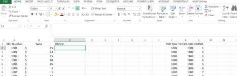
I want C2 to return the value in column L if A2 is found in either column J or K). In this case, C2 would be 1. The other example with the "or" as in C22 would be 2 (as the total is found in column K). Is that possible? Your help is greatly appreciated. Thank you in advance.

 

[Fluff]

What version of Excel are you using?

I suggest that you update your Account details (or click your user name at the top right of the forum) so helpers always know what Excel version(s) & platform(s) you are using as the best solution often varies by version. (Don’t forget to scroll down & ‘Save’)

 

[atoice]

Sorry - thanks for your reply. it's excel 2013. I'll drop it in.

 

[Fluff]

Thanks for that.
How about

=INDEX($L$2:$L$100,IFNA(MATCH(A2,$J$2:$J$100,0),MATCH(A2,$K$2:$K$100,0)))

 

[jtakw]

Hi,

Another way:

Book3.xlsx
	A	B	C	D	E	F	G	H	I	J	K	L
1
2	1001		1							1001	1001	1
3	1002		2							1002	1102	2
4	1003		3							1003	1103	3
5	1004		4							1004	1104	4
6	1005		5							1005	1005	5
7	1006		6							1006	1106	6
8	1007		7							1007	1007	7
9	1008		8							1008	1108	8
10	1009		9							1009	1009	9
11	1010		10							1010	1010	10
12	1011		11							1011	1011	11
13	1012		12							1012	1112	12
14	1013		13							1013	1113	13
15	1014		14							1014	1114	14
16	1015		15							1015	1015	15
17	1016		16							1016	1016	16
18	1017		17							1017	1017	17
19	1018		18							1018	1118	18
20	1019		19							1019	1119	19
21	1020		20							1020	1020	20
22	1102		2
Sheet1020

Cell Formulas
Range	Formula
C2:C22	C2	=LOOKUP(2,1/FIND(" "&A2&" "," "&J$2:J$21&" "&K$2:K$21&" "),L$2:L$21)

 

[atoice]

Hi Jtakw! JACKPOT! Thank you so much for your quick reply. I did try using Find as well, and no luck. I didn't know Lookup could be used alone. V/H/or X.

Would this apply to if the columns were on another tab for Lookup/Find, correct?

Have a great weekend.
MT

 

[jtakw]

You're welcome, thanks for the feedback.

 

[jtakw]

At OP's request, here's an explanation of my formula in Post # 5.

The LOOKUP function is looking for the value of 2 within the "lookup vector", which, in this case is:

1/FIND(" "&A2&" "," "&J$2:J$21&" "&K$2:K$21&" ")

We want to find the value of A2 (e.g. 1001) in either Column J or Column K,

So I used the FIND function (case sensitive, but since we're dealing with numbers, makes no difference) but added a Space before and after the value of A2 (e.g. " "&A2&" "), so A2 becomes " 1001 "

I also concatenated Column J and Column K, Also adding a Space before, in between, and after the Column J & K values per row (e.g. " "&J$2:J$21&" "&K$2:K$21&" "), so J2:K2 becomes " 1001 1001 ", J3:K3 becomes " 1002 1102 ", and so on for Each row.

The reasoning behind adding the Spaces is to avoid the possibility of erroneous results from values like:
A2=1011, J2=1010, K2=1102
Without the addition of the spaces, J2&K2 becomes "10101102" which Does contain "1011", and the FIND function will interpret that as a Match
With the addition of spaces, J2&K2 becomes " 1010 1102 " which does Not contain " 1011 ", so it's Not a Match.

So now, 1 is divided by the results of the FIND function, thereby, making the FIND results Never larger than 1

LOOKUP is looking for 2 within a vector that Only contains numbers that are 1 or smaller and #VALUE! errors,
LOOKUP will ignore the errors, but can't find the 2, so it resolves to produce the Last instance of a number Smaller than 2
and produces the Position of this value within the "result vector" in the formula L$2:L$21

My formula in Post # 5

=LOOKUP(2,1/FIND(" "&A2&" "," "&J$2:J$21&" "&K$2:K$21&" "),L$2:L$21)

Does Not have to be written with the "2,1/" part, bold in red above, it could also be written as:

=LOOKUP(9.99999999999999E+307,FIND(" "&A2&" "," "&J$2:J$21&" "&K$2:K$21&" "),L$2:L$21)

where we use the commonly referred to as BIG NUM (the largest number Excel will recognize), the principle is the same.
Some excel users my use something like 9^9 or 2^15, rather than the BIG NUM, there are instances where these values will suffice for the purpose of the calculation, but may Not work in All instances.

Hope this helps.